Persistent Scaffold Computation:
Causal Presentations, Sewing, and Feedback
Expanded reading edition · 5 September 2026; qualification alignment · 7 October 2026
When two construction histories mean the same thing
A persistent graph records how it was built. An observer at its newest node may see only a small part of that record. This article asks which changes to the construction preserve what such an observer can learn, and how those changes can be composed.
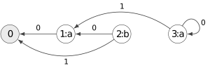
Start with three nodes, each with one outgoing edge. Node 1 has label
1 and points to itself. Node 2 also has label
1 and points to node 1. Node 3 has label 0;
when created, it copies node 2’s outgoing endpoint, so it points to node
1. Looking forward from the final root, an observer sees 0,
then 1 forever.
Node 2 is unreachable from that final root. Nevertheless, its edge was consulted when node 3 was created. Erasing node 2’s label has no effect on the final graph. Changing its edge before replaying the construction may change where node 3 points. Unreachable information and information irrelevant to replay are therefore different notions.
That example motivates causal support: keep the labels and edges visible in the final graph, then also keep every earlier edge that was used to compute a kept edge. Repeat until all such dependencies have been included. Everything outside this support can be changed without affecting replay. The proof follows those dependencies in chronological order.
The article also distinguishes two ways for histories to agree. They may give the same observable graph at every intermediate time, or only at the final time. The first is stronger. A change that moves a useful record from an earlier node to a later node can preserve the final answer while changing what was visible midway through the construction.
For the stronger equivalence, two local moves suffice. An endpoint detour replaces one path description by another path reaching the same old node. An absorption gives a new node its own self-loop when it already presents the same recursive behavior as an older self-looping node. The proof shows that repeatedly applying these moves reaches one canonical history for each complete sequence of observations.
Final observation allows more freedom. Some labels become irrelevant; useful records can move between construction times. In the case of one outgoing edge and distance-one access, these movements admit a particularly concrete description. Place the essential records in increasing time order, with the final root fixed at the final time. A move shifts one record into a neighboring vacancy. The legal placements form an order-ideal lattice, whose commuting moves give a cube geometry.
This geometric description is a theorem about histories and their relationships. It does not automatically give an automaton a procedure for discovering equivalent histories or normalizing them while input arrives. The distinction matters to the later residual-access result: a compact semantic description and an inexpensive update procedure are separate achievements.
The final section returns to computation. It shows how bounded batches of logical records, including fresh cycles, can be represented by one scaffold node per input symbol. The same finite slot technique appears in the direct-palindrome construction. Its current Draft 5 direct theorem is conditional on the complete Section 11.1 sequence contract; the concrete implementation remains informal evidence with open source-contract obligations, and numerical radius/distance remain withdrawn. The follow-up unary coherence article goes further in another direction: it compares whole sequences of history transformations, rather than only their endpoints.
1 From a finite presentation to a history algebra
1.1 The machine and the question
Loff, Moreira, and Reis (LMR) introduced scaffolding automata as a machine model for parsing expression grammars [12]; Section 2 defines both. For now the picture suffices. At each input position the machine reads a fixed-radius neighborhood of the current top of a persistent graph, chooses a finite label, and appends one new node. Each new edge is missing, points to the fresh node itself, or follows a bounded path from the preceding top. LMR prove that a language has a PEG if and only if its reversal is decided by such a machine [12, Theorem 16].
The usual observation made of such a machine is acceptance: does the run end in an accepting state? This paper keeps more of the generated object visible. A run has a physical graph at every time; an observer standing at the top and following edges sees, at every time, a behavioral figure; and at the end there is a final figure. Those are different quotients of the same history, and the paper’s question is:
When two finite construction histories generate the same behavior, which local fold, unfold, routing, erasure, and feedback moves connect them?

The answer has two layers. For every fixed finite degree and observation distance, two graph-local rewrites give a terminating, confluent presentation of the histories that have the same behavioral figure after every prefix (Theorem 6.8). Equality of only the final figure is harder because it forgets intermediate behavior; we prove what we can (Section 7–8) and state exactly what remains open (Section 10).
1.2 In what sense this is an “algebra”
We call the system of histories, behavioral equivalences, and rewrites an algebra in the informal sense in which one speaks of “the algebra of regular expressions”: a collection of objects, operations on them (appending a row, rewriting a row), and equations between the results. Where a formal algebraic structure is meant, it is named and proved: the monoid of rows under concatenation (Section 3), the transformation monoid of port navigation and its -triviality (Corollary 4.2), and the rewriting system with its normal forms (Theorem 6.8). No claim is made that the calculus is an instance of any particular variety, category, or polygraph; whether it is, is an open comparison (Section 10).
1.3 What is new here, and what is inherited
The paper leans on three established theories and does not rename them. Bisimulation (two states are equivalent when every observation and every successor behavior matches) and the quotient of a system by it are standard objects of coalgebra [15, §2, §5–6]; the familiar instance is the minimal deterministic automaton obtained from the residuals (derivatives) of a language [3, 13]. Bottom-up merging of equivalent states and incremental minimization of acyclic deterministic automata are established [5, §2]. Cyclic term graphs, their unwinding into infinite trees, copying, hidden nodes, and confluence have a substantial theory [2]. Section 11 lists what is inherited from each.
The target here is the intersection of four restrictions that none of those theories imposes together:
one immutable layer is appended per input symbol;
every old address is read from the preceding top within one fixed radius;
a strong move must preserve the figure after every prefix; and
soundness must survive every common future continuation.
The resulting local rules live in the generated scaffold graph. They need not be bounded contiguous substring rules in the linear word of rows.
1.4 The viewpoint
Finitely Presented Recognition Dynamics, abbreviated FPRD, is the research viewpoint used in this work: a finite grammar or machine description is treated as a presentation that generates an internal recognition dynamic, and the accepted language is treated as one observation of that dynamic. FPRD Lab is the AI-assisted research project in which the present arguments were developed; nothing in this paper requires trust in that project, and Section 11 states plainly what was checked and by whom. In this paper the viewpoint has a concrete form, Figure 1: changing an observation may merge histories without changing the rows that generated them; changing a presentation may alter the physical history while preserving every behavioral figure. The algebra begins by keeping both phenomena explicit.
1.5 How to read this paper
Section 2 supplies the background: words and languages, context-free grammars and PEGs, LMR’s scaffolding automaton with a drawn example, and the step from automata to arbitrary construction histories, which is where this paper’s objects begin. Section 3 defines histories, unfoldings, figures, and the two equivalences, with one worked history that recurs throughout. Sections 4–6 develop the strong-trace calculus: the chain theorem, guarded folds, and the two rewrites with their normal form. Sections 7–8 treat final observation. Section 9 gives the feedback application. Sections 10–11 state open problems, what is inherited, and how the work was produced. Every proof states its strategy first; every example says what generalizes.
2 Background
2.1 Words and languages
An alphabet is a finite set of letters; a word is a finite sequence of letters, is the empty word, and is the set of all words over . A language is a set of words. The reversal of is . A monoid is a set with an associative operation and an identity; under concatenation, with identity , is the free monoid on : every word is a unique sequence of letters.
2.2 Context-free grammars and parsing expression grammars
A context-free grammar has terminal symbols, non-terminal symbols, a start symbol, and rewriting rules with one non-terminal on the left [4, pp. 120–122]; it generates the words obtainable from the start symbol by repeatedly replacing a non-terminal by a right-hand side. For instance generates the even-length binary palindromes . The reading is existential: a word is in the language if some derivation produces it.
A parsing expression grammar (PEG) [7, §3] uses similar rule shapes with an operational meaning. Expressions are built from letters, non-terminals, , and by sequence , ordered choice , and the predicates and ; each non-terminal has one rule . Recognition reads from the left and either fails or succeeds consuming a prefix: a letter consumes itself; a sequence runs its parts in order; ordered choice runs and commits to it if it succeeds, trying only if fails; succeeds (consuming nothing) exactly when fails [12, Definition 3, Algorithm 1]. The procedure is deterministic. A grammar is total if recognition never loops, and the language of a total grammar is , the words on which the start symbol succeeds consuming the whole input (“complete match”); is the class of such languages [12, Definition 4]. Order is semantic: with , the input is not recognized, because the choice commits to and leaves unconsumed [7, p. 7]. PEGs recognize some non-context-free languages, such as [12, p. 3], while LMR conjectured that the context-free language has no PEG [12, Conjecture 7]; the comparison of the two classes is not syntactic and goes through the machine model below.
2.3 Scaffolding automata
Definition 2.1 (scaffold [12, Definitions 10–11]). Let and let be a finite alphabet. A -scaffold with top has nodes ; a label for each node, with (the base is unlabelled); and for each node and each port a target : every edge points to an older node or to the node itself, or is missing. A port word is followed from a node by taking port , then port of the node reached, and so on; it is valid from if no missing port is met. The -neighbourhood is the labelled tree of depth obtained by unfolding ports from ; it records labels and missing ports, not node numbers.
Definition 2.2 (scaffolding automaton [12, Definitions 12–15]). A scaffolding automaton has an input alphabet, a degree , a working alphabet , a distance , a finite control , and a transition function . Reading a letter in state with top , it computes and appends node with label and ports: the endpoint of followed from if is a valid port word; missing if or invalid; the new node itself if . It accepts a word if the state after the last letter is in .
Theorem 2.3 (Loff–Moreira–Reis [12, Theorem 16, p. 21]). A language is in if and only if is decided by some scaffolding automaton.
The reversal is not an artifact: the automaton commits letter by letter from the left, and LMR’s grammar re-enacts its run from the other end. This paper uses the theorem only in the labelled example of Section 9; none of its own results depends on it.
2.4 From automata to histories
Everything from Section 3 to Section 8 concerns the graphs that scaffolding automata can build, not any particular automaton. A run of an automaton on an input word writes down, at each step, one row: the label chosen and the descriptors chosen. Conversely, any sequence of rows is a legal construction (an invalid port word simply yields a missing edge), whether or not some finite control would produce it. We therefore study all finite row sequences, called histories, and ask about their behavior as seen by an observer at the top. The finite control, the input word, the distance bound on what the control may read, and acceptance play no role until Section 9. In particular the rewrites of Sections 6–8 are mathematical operations on histories; we do not claim that an automaton could perform them while running (Section 6.3 says this once more where it matters).
3 Histories, unfoldings, and observations
3.1 The finite row alphabet
Fix a degree , a distance , and a finite working alphabet . Write for the port alphabet and for the set of descriptors.
Definition 3.1 (row, history). A row is an element of : one label and one descriptor per port. A history is a finite sequence of rows. The empty word is a valid descriptor: it names the preceding top.
Definition 3.2 (Evaluation). A history is evaluated from an unlabelled edgeless base node . At time , append node with label . Its port is missing if , points to if , and otherwise points to the endpoint obtained by following from node in the old scaffold. An invalid path gives a missing edge. We write for the scaffold after the first rows.
The set of histories is the free monoid as syntax. Appending a row is a total operation on evaluated histories because invalid paths have the defined missing outcome.
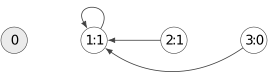
Example 3.3 (a worked history). Take , , , so every descriptor is one of , , , (the only port word of length ). The history evaluates as follows (Figure 3). Row 1 creates node with label and a self-loop. Row 2 creates node with label pointing to the old top, node . Row 3 creates node with label whose port follows port word from node : node ’s port leads to node , so node points to node . Node is not reachable from node , yet its port cell was consulted when node ’s edge was evaluated; this distinction drives Section 7. What generalizes: every history is evaluated this way, one row at a time, reading only the previous top’s surroundings. What is incidental: the labels and the length.
3.2 Port-word behavior
For a rooted evaluated scaffold , following a port word from either reaches a node or runs into a missing port. Adjoin a value for the latter. The behavioral unfolding of is the function that sends a valid word to the label of its endpoint (with for the base) and an invalid word to . The unlabelled base is therefore observable and is not a missing edge. The unfolding is everything an observer at can learn by following ports and reading labels; it is what LMR’s transition function sees, restricted to words of length at most .
Two rooted scaffolds are behaviorally equivalent, written , when their unfoldings agree. For a history of length , let denote the canonical minimal figure of its length- prefix, defined in Section 3.4. The strong trace and final observation are
Definition 3.4 (Two congruences). Equal-length histories are strongly equivalent, , when . They are finally equivalent, , when .
Strong equivalence implies final equivalence. The converse fails because a later row may make an earlier difference unreachable or behaviorally irrelevant.
Example 3.5. With , the histories have the same final figure—a single node labelled with a missing port—because in the second history every descriptor follows a port that is itself missing. Their strong traces differ already at time (labels versus ). Many histories share a final figure while their strong traces differ; the displayed pair is the smallest fact used below.
3.3 Full abstraction
The first theorem says that the unfolding is the right notion of behavior: it is determined by finite observations, it is exactly bisimilarity, it is preserved by every common future, and any difference is eventually visible.
Theorem 3.6 (Future-context full abstraction). For rooted degree- scaffolds over one working alphabet:
equal unfoldings, equality of every finite rooted neighborhood, and deterministic labelled bisimilarity are equivalent;
unfolding equivalence is preserved by every common scaffold row and hence by every common continuation; and
unequal unfoldings are distinguished after finitely many steps by a distance-two unary scaffold continuation.
Here a bisimulation between two rooted scaffolds is a relation on nodes that relates the roots and, whenever it relates to , requires that and have the same label and that for every port either both are missing or the targets are again related; two roots are bisimilar if some bisimulation relates them. “Unary” means that the continuation uses only one port of each new node; “distance two” means its descriptors have length at most (whatever the distance of the original scaffolds). “Distinguished” means: there is a single sequence of rows which, appended to either scaffold, produces tops whose depth- neighbourhoods differ, so that a finite control reading those neighbourhoods can accept one and reject the other.
Proof. Strategy. (1) is a restatement; (2) is an induction on the query word; (3) constructs a “cursor” that walks along a shortest distinguishing port word, one letter per row.
The depth- neighborhood is exactly the restriction of the unfolding to port words of length at most , which proves the first equivalence. The relation “same unfolding” is a bisimulation, and conversely a bisimulation forces equal unfoldings by induction on the word.
Suppose the old unfoldings agree and append the same row. The observed depth- neighborhoods agree. For a query word starting at fresh port , a missing descriptor fails on both sides; a descriptor returns to the respective fresh root; and an old descriptor reduces the comparison to . The fresh labels agree. Induction on the remaining query length proves equality of the new unfoldings. Iterating proves continuation stability.
For the converse, choose a shortest port word on which the unfoldings differ. If , the current labels already differ. Otherwise a unary tester stores a cursor in one port. Its first row points along ; at the next step the distance-two path through the cursor and advances it; and so on. All proper prefixes behave identically by minimality. The last neighborhood exposes the first label or missing-edge difference, which finite control records in acceptance. ◻
Corollary 3.7. Both and are stable under a common right suffix of rows.
3.4 Why coalgebra, and what a figure is
The reader who knows finite automata has met the idea of this subsection already. A language has, for each word , a residual (or derivative) ; the language is regular exactly when it has finitely many residuals, and those residuals are the states of its minimal deterministic automaton [3, Def. 3.1, Thm. 4.3], [13]. Two states of any automaton are equivalent when they accept the same words, and merging equivalent states gives the minimal automaton. Coalgebra is the general form of this idea: a system is described by what can be observed at a state (here, a label) and which states are reached next (here, the port targets); two states are bisimilar when every observation and every successor behavior matches; the quotient by bisimilarity is the smallest system with the same behavior [15, §2, §5–6]. We use only this much of the theory, in the deterministic labelled-graph instance, and we prove the facts we need directly.
For a valid port word , write for the residual unfolding at : what an observer sees after first walking along . Let be the finite set of distinct valid residual unfoldings. A map from the nodes of one rooted labelled port graph to those of another is a functional bisimulation if it sends root to root, preserves labels, and for every node and port either both and lack port or . Two rooted labelled port graphs are isomorphic if there is a bijective functional bisimulation between them.
Theorem 3.8 (Minimal residual figure). Every finite rooted scaffold has a canonical finite behavioral figure whose states are , whose root is , and whose port sends to when defined. The physical reachable graph maps onto by a surjective functional bisimulation. Two rooted scaffolds are behaviorally equivalent if and only if their minimal figures are isomorphic.
Proof. Every residual is represented by a physical reachable node, so there are at most as many residuals as nodes. Residualization commutes with every port ( implies ), which makes labels and successors well defined and makes the node-to-residual map a functional bisimulation. Distinct residual functions have distinct unfoldings and cannot be bisimilar. The construction depends only on , proving minimality and uniqueness up to rooted labelled port-graph isomorphism. ◻
Example 3.9. For the worked history of Example 3.3, the residuals from node are: (label , then forever) and (label forever). The figure has two states, a -labelled root pointing to a -labelled state with a self-loop. The physical node is not reachable and plays no part.
Remark 13. Physical aliasing is finer than behavior. Two ports may point to one node in one history and to two bisimilar nodes in another; their minimal figures still agree. Alias identity becomes observable only when a presentation explicitly stores it in finite labels.
4 Chronological order and navigation
Write when is reachable from by following ports, including ; since edges point to older nodes or to the node itself, implies that was created no later than , so later nodes sit above earlier ones. A finite port graph is weakly acyclic when its only directed cycles are self-loops. Its rooted component is a reachability chain when is a total order there.
Theorem 4.1 (Generated-chain theorem). Let be a legally generated chronological scaffold with current top .
Its physical graph and its minimal figure are weakly acyclic.
The nodes reachable from , and the states of the minimal figure, are totally ordered by reachability.
Conversely, every finite behaviorally reduced labelled rooted reachability-chain port graph, with an optional least unlabelled edgeless state, has an exact legal scaffold presentation at some finite distance.
Part (2) is worth a pause: it says that, from the top, any two reachable nodes are comparable, one reachable from the other. The reason is that a new node can only point into the previous top’s reachable set, which is a chain by induction.
Proof. A non- edge of node reaches an older node, so creation time never increases along a port path and can stay fixed only on a self-loop. If the behavioral quotient had a cycle through two classes, repeating a word around the cycle from a physical representative would give an infinite path of nonincreasing times. It is eventually constant, so every later edge is one physical self-loop and all classes on the alleged cycle coincide.
Let be the component reachable from the top after step . Every old target of the new top is already in , so . Induction makes a chain, and quotienting preserves total comparability.
Conversely enumerate the desired states . When is appended, each strict successor is some at or below and is therefore reached from by a port word. Use that word, for self-loops, and missing for absent edges. A shortest simple word has length at most , so one distance at most realizes all rows. ◻
A transformation of a finite totally ordered set is regressive if for every (we write the action on the right). In a monoid , Green’s relation is defined by iff , i.e. and for some ; is -trivial when every -class is a singleton [14, Ch. V §1, p. 99; Ch. X §1.3].
Corollary 4.2 (Regressive navigation). After adjoining a least missing sink to a generated minimal figure and numbering its chain, every port acts regressively. Its port-word transition monoid is a submonoid of the full regressive transformation monoid and is -trivial.
Proof. Each successor is at or below its source. If transformations are -related, write and . Pointwise regressiveness gives and for every state , hence . ◻
Boundary. This is the algebra of historical port navigation inside one figure. It says nothing about the streamed input language, and nothing about the finite control’s routing of roots, which is a separate finite interface.
5 Static guarded folding
5.1 Rewriting vocabulary
A rewriting system on a set is a binary relation (“one step”). An object is irreducible, or a normal form, if no step applies to it. The system is terminating if there is no infinite sequence of steps, and confluent if whenever an object rewrites (in zero or more steps) to two objects, those two rewrite to a common object. A terminating confluent system gives every object exactly one normal form, and two objects are related by the equivalence generated by exactly when they have the same normal form; this is the Church–Rosser property. We use these words in exactly this sense.
5.2 Guarded folds
Let be a finite deterministic labelled partial port graph and let be a bisimulation equivalence already imposed on it (an equivalence relation that is a bisimulation). Work in the quotient , whose states are the classes and whose ports are well defined because is a bisimulation.
Definition 5.1 (Elementary guarded fold). Two distinct quotient states admit a guarded fold when their labels agree and, at every port, the two successors are both missing, are the same quotient state, or lie in . Equivalently, identifying and makes their one-step successor profiles equal.
The last case is the guarded recursive clause. It permits self-reference at either member of the pair but no larger unresolved cycle.
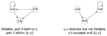
Theorem 5.2 (Guarded folds generate bisimilarity). On every finite weakly acyclic deterministic labelled partial port graph, the equivalence generated by elementary guarded folds is exactly the greatest bisimulation equivalence.
Proof. Strategy. Soundness is immediate. For completeness, find, in any sound quotient that is not yet fully reduced, a bisimilar pair that satisfies the guard: take a minimal unreduced class and look at its sinks.
Each fold is sound because corresponding successors become equal in the new quotient.
Two facts keep the induction well posed. First, the greatest bisimulation quotient of a finite weakly acyclic graph is weakly acyclic: the argument of Theorem 4.1(1) applies verbatim with any topological numbering in place of creation time. Second, a guarded fold preserves weak acyclicity: a new cycle through the folded class would pass through a state that is a successor of or and reaches or ; since and have identical non-pair successors, is a successor of both, so the old graph had a cycle of length at least two, contradicting weak acyclicity. Hence every sound quotient reached by folds is weakly acyclic, and “minimal in strict reachability” below is meaningful.
For completeness, suppose a sound quotient still has a nonsingleton greatest bisimulation class. Choose such a class minimal in strict reachability of the behavioral quotient. Every strict successor class below is already a singleton.
The edges between distinct current states inside form a finite DAG. If it has two sinks , an internal successor of either sink can only be its own self-loop, while corresponding external successors are the same singleton; therefore are guarded-foldable. If it has one sink , choose a minimal state of . Every strict internal successor of is , and every internal successor of is its self-loop. External successors are again equal, so are guarded-foldable.
Another sound fold is therefore available until the greatest bisimulation quotient is reached. ◻
Corollary 5.3 (Static normal form). Orient each guarded fold toward its quotient. The system terminates and is confluent up to rooted labelled port-graph isomorphism. Its normal form is the minimal residual figure.
Proof. Every fold reduces the state count. An irreducible graph is behaviorally reduced by Theorem 5.2; every reduction preserves the unfolding; and Theorem 3.8 gives one reduced figure up to isomorphism. ◻
This theorem contains the usual bottom-up acyclic merge [5, §2] as a special case. The extra local case is a self-recursive pair. Static normalization alone, however, may remove a physical state and therefore does not yet define a time-respecting rewrite of construction histories: the next section asks which rewrites of the rows realize it.
6 The causal presentation calculus
6.1 Strong equivalence and semantic sewing
A semantic step replacement changes one row over a fixed preceding prefix when the two possible fresh roots are behaviorally equivalent.
Proposition 6.1 (Semantic causal sewing). Two strongly equivalent length- histories are connected by at most semantic step replacements.
Proof. Align the rows from left to right. Once the prefixes through are literally equal, replaying the old th row over that prefix preserves its behavior by Theorem 3.6; the target row has the same th figure by strong equivalence. Replace it and continue. ◻
So there is no semantic obstruction: strongly equivalent histories are always connected by row replacements. The real problem is locality: the side condition “the two fresh roots are behaviorally equivalent” is a global statement about unfoldings, and we want a fixed family of moves each of which is justified by looking at a bounded piece of the scaffold.
6.2 One-state extensions
Let be a behaviorally reduced old live figure (the reachable part of the old scaffold, assumed to have no two bisimilar nodes). It is convenient to describe a new row not by descriptors but by what its ports reach: a new row has the guarded one-variable form where denotes the fresh root itself. We say the fresh root presents a behavior, namely its unfolding; it presents an old residual if its unfolding equals that of .
Lemma 6.2 (One-state extension dichotomy). Suppose two such fresh roots have the same behavior.
If the behavior is not already a state of , their missing and positions agree, and their old target agrees at every other port.
If the behavior is an old state , each row is a guarded unroll of : it copies every missing and strict-successor port, while a self-loop of may target either or the fresh variable .
Proof. In the first case, a fresh on one side and an old target on the other would make the common fresh behavior equal to , a contradiction. Thus the masks agree. Corresponding old targets are bisimilar and are therefore the same state of reduced ; missing positions also agree.
In the second case, compare the fresh root with . A non- target must be the unique reduced successor of . A fresh is possible exactly where that successor is itself. These conditions are also sufficient: identity on together with the fresh-root/ pair is a bisimulation. ◻
6.3 The two primitive strong moves
Fix the total order on descriptors, where port words are ordered by length and then lexicographically (so is the least port word), and order rows with the same label by comparing descriptor tuples position by position.
Definition 6.3 (Endpoint detour ). Replace one old-top word by another bounded word with the same physical endpoint. All invalid words share the missing endpoint. Orient the move toward the least name of that endpoint.
Definition 6.4 (Literal guarded unroll ). Let a fresh row point, at some port, to an old physical node that has a self-loop at that port, and suppose the fresh root presents the residual of : its label equals ’s, and at every port its target is missing exactly when ’s is, is the physical successor of where that successor is not , and is either or where has a self-loop. If at least one such port points to the old , replace all of them by and choose least endpoint names at the other ports. Orient in that direction.
The simultaneous recursive part of is absorption ; its remaining changes are endpoint detours. The guard is physical and bounded: it names within the observed scaffold and inspects its fixed port tuple.
Example 6.5 (the two moves on the worked history). In , row 2 points to node , which has a self-loop and the same label, and node ’s unfolding equals node ’s; so applies and rewrites row 2 to . After that rewrite, row 3’s descriptor is followed from the new node , whose port is now a self-loop, so the endpoint is node ; the least name for node from the old top is , and rewrites row 3 to . The result has the same figure as at every time. What generalizes: an unroll can change the physical endpoints of later rows, and detours then rename them.
These are mathematical graph-local rewrites with explicit endpoint-equality certificates. The calculus does not assert that an LMR automaton can discover or execute a normalizing move from finite control, nor that the move occupies a bounded contiguous interval in the chronological row word.
6.4 SELF-eager prefixes
Call a canonical history SELF-eager when it uses at every available self-loop coordinate and least names elsewhere; by the order fixed above, this is the same as being the least row at every step.
Lemma 6.6 (Canonical history exists). Every realizable finite strong trace has a unique lexicographically least history. It is obtained from left to right by appending the least row that realizes the next figure over the already chosen prefix.
Proof. Assume the canonical prefix through time has been chosen and take any original realization of the full trace. Its length- prefix has the same rooted unfolding as the canonical prefix. Replay the original th row over the canonical prefix. Theorem 3.6 says that the new root has the required th figure, so the finite set of realizing rows is nonempty and has a unique least element. Induction constructs the history; leastness at the first differing row proves uniqueness. ◻
Lemma 6.7 (Reduced live prefixes). Every root-reachable component at every prefix of a SELF-eager history is behaviorally reduced.
Proof. Induct on prefix length. If the fresh behavior is new, it adds one new residual above a reduced old component. If it repeats an old residual , Lemma 6.2 says that every strict successor lies below and that only a self-loop coordinate can choose between old and fresh . SELF-eagerness chooses the fresh root. It therefore reaches itself and strict descendants but not the old physical . The fresh root replaces as the unique live representative. ◻
Theorem 6.8 (Convergent strong-trace presentation). For fixed finite , oriented endpoint detours and literal guarded unrolls form a terminating confluent graph-local presentation of strong equivalence. Two histories have the same strong trace if and only if they reduce to the same SELF-eager history. A length- history normalizes in at most row moves when counts as one whole-row move.
Proof. Strategy. Soundness of each move; termination by a lexicographic measure; then show that an irreducible history is the canonical one of Lemma 6.6, by induction from left to right.
Both moves are sound. A detour preserves a physical endpoint. For an unroll, identity on the old prefix together with the fresh-root/ pair is a bisimulation. Theorem 3.6 carries either replacement through the unchanged suffix.
Lexicographically order the chronological descriptor word. A detour strictly decreases one path name. An unroll replaces at least one old path by smaller and never increases an earlier descriptor. Thus reduction terminates.
Induct left to right through an irreducible history. Its old prefix is already SELF-eager and reduced by Lemma 6.7. Compare the fresh row with the least row supplied by Lemma 6.6 for the same next figure. If the residual is new, Lemma 6.2 gives the same missing/ mask and the same old residual targets. Reducedness turns those targets into the same physical nodes; any remaining difference is a detour redex. If the residual repeats old , a path back to at a self-loop is an unroll redex, and a nonleast path to any fixed strict successor is a detour redex. Therefore an irreducible row is exactly the SELF-eager least row.
Each strong-trace class has one irreducible history, so termination gives confluence and completeness. Normalizing from left to right, a new residual needs at most detours. A repeated residual needs at most detours or one whole-row unroll; because , the total is at most . ◻
Remark 27 (What “coherence” means here). Theorem 6.8 is object-level Church–Rosser coherence: equal strong traces have one normal form, so any two reduction sequences from one history end at the same place. It does not say that any two such sequences are themselves related by a finite list of elementary identities between sequences (“two-dimensional cells”). We reserve the phrase path-level coherence for results that actually present those relations between sequences of moves.
7 Final observation and replay support
Final equivalence forgets intermediate figures. A row that is unreachable in the final rooted graph can nevertheless have been queried while a later descriptor was evaluated: in the worked history , node is not reachable from node , but node ’s descriptor was evaluated by reading node ’s port. Ordinary graph garbage (unreachable nodes) is therefore too small a notion of “irrelevant data”; the right notion follows the evaluation.
We call the descriptor written in row a port cell and the label a label cell; these are the syntactic coordinates of a history. Evaluating a port cell that holds a port word from the old top queries the port cells of the nodes it passes through, including the one at which an invalid path fails.
Definition 7.1 (Causal endpoint support). Let be the created nodes reachable from the final top. Support every label cell and every port cell of a node in . Whenever a supported port cell was created by following an old-top path, support every older port cell actually queried along that evaluation, including the cell at which an invalid path fails. Close backward to the least such set .
Example 7.2. For : ; the supported label cells are those of rows and ; the supported port cells are those of rows and and, because row ’s descriptor queried node ’s port, also the port cell of row . Row ’s label is unsupported.
Theorem 7.3 (Replay invariance). Suppose an equal-length history agrees with on the labels of and on every descriptor cell in . Then the final rooted concrete scaffolds of and are identical. Moreover and .
Proof. Proceed chronologically through supported descriptor cells. Every dependency of a supported cell is an earlier supported cell, so induction makes its evaluation traverse the same physical endpoints on both sides. The outgoing edges and labels of all final-reachable nodes are therefore identical, giving the same rooted concrete scaffold and the same reachable set. Recomputing the least backward closure follows the same descriptor traces, hence gives the same support. ◻
Definition 7.4 (Garbage fibre). is the set of histories agreeing with on the data named in Theorem 7.3. A -move changes any collection of the remaining data.
Theorem 7.5 (Causal-garbage cube). Every garbage fibre is the Cartesian product of the finite value sets of its unsupported label and descriptor coordinates. Simultaneous factors into single-coordinate changes. Fill a triangle for three values of one coordinate and a square for changes of two distinct coordinates. The resulting path two-complex is simply connected.
The last sentence is a statement about sequences of garbage moves, of the kind Remark 6.9 calls path-level: form the graph whose vertices are the histories of the fibre and whose edges are single-coordinate changes, glue in a two-dimensional face for every triangle and every square named in the theorem, and the claim is that every closed loop of moves can be contracted across those faces—any two ways of making the same garbage change are related by the displayed elementary identities.
Proof. Support stability in Theorem 7.3 makes every unsupported coordinate independent. Order the coordinates. Commuting squares move all changes of the first coordinate to the front, then the second, and so on. Same-coordinate triangles compose each block to the direct change between its endpoint values. Every path reduces to one coordinate-ordered path; a loop reduces to the empty path. ◻
7.1 A noncommuting boundary
Let denote strong normalization (Theorem 6.8) and let (“junking”) choose least values outside causal support. Both preserve the final figure, but in general An absorption can move a repeated residual to a newer physical carrier. Junking first may erase the label needed to perform that absorption; absorbing first makes the older carrier garbage. Thus the two normalizers can reach distinct common fixed points with one final figure already in the unary distance-one three-row fragment.
Concretely, take the worked history .
| row 1 | row 2 | row 3 | comment | |
|---|---|---|---|---|
| node ; node unreachable but queried | ||||
| row 2 absorbed; row 3 renamed to the new carrier | ||||
| row 1 now entirely garbage | ||||
| row 2’s label unsupported, set to ; its port cell kept | ||||
| already strong-normal: node no longer presents node |
Both final roots are labelled and point to a -labelled self-loop, but and are distinct and irreducible under both normalizers.
Boundary. Object-level confluence for strong traces plus cubical coherence inside each garbage fibre does not present their join. The missing operation changes which chronological node carries a final residual and therefore changes the support boundary itself.
8 Two calibrated sewing theorems
This section does not assert a complete final-equivalence calculus at arbitrary degree and distance. It proves one local two-row theorem and one global unary theorem. Their different hypotheses show where the remaining problem lies. “Sewing” is used literally: given two histories with the same final figure, we want a sequence of local moves that stitches one into the other while every move preserves the final figure.
8.1 Unexposed acyclic two-row factorizations
Fix a behaviorally reduced old prefix with top , append one node (the router), then one more node (the consumer). The router’s ports are its slots. A consumer port whose descriptor is a nonempty port word is a path demand; its first letter is its selector, naming router slot . Assume no consumer port points to by the empty descriptor. Whenever a consumer word begins with router slot , assume that slot contains an old-prefix path , not or missing. Thus a consumer word reaches the node reached from by the composite word . Call such a block unexposed (the consumer does not point at the router itself) and acyclic (the used slots point into the past). Because every consumer port points into the old prefix, the router is unreachable from and hence from every later top: no later row can see or query . Consequently ’s label and its unused slots are outside causal support, while a slot used by some consumer demand is queried and supported.
Three final-only moves are useful.
A routing crossing injectively reassigns used router slots and changes each first selector to follow the reassignment.
A cut slide moves one letter between and when both bounded descriptors remain legal.
A dedicated relation exchange changes to in a slot selected by exactly one consumer port, under the guard .
The first two refactor a fixed composite word. The third uses a relation in the pointed old navigation action and is the move that crosses between different words with one old endpoint.
Theorem 8.1 (Unexposed two-row sewing). Fix , , and a behaviorally reduced old prefix. Consider two unexposed acyclic two-row extensions with the same consumer label, the same valid nonmissing path-demanding consumer coordinates, and literal agreement as missing or on every other consumer coordinate. If corresponding path demands have the same final old residual behavior, the blocks are connected by endpoint detours, causal-garbage moves, continuation-aware routing crossings, and dedicated relation exchanges. Every common suffix is preserved.
Here “the same final old residual behavior” means that the nodes reached in the old prefix by corresponding demands have equal unfoldings, and “continuation-aware” records that a routing crossing rewrites the consumer’s selectors together with the router’s slots; in the present setting no later row can reach the router, so the common suffix is literally unchanged.
Proof. Strategy. Make each demand own a private router slot, then change the slots one at a time under the endpoint guard, then undo the private splitting.
Reducedness makes equal old residual behaviors the same physical old state. Canonicalize every missing consumer coordinate to literal missing by a detour.
If several path demands use one first selector, fewer router slots than demands are currently used. Copy that router descriptor into an unsupported slot by (legal, since unused slots are outside support) and retarget one consumer word to the copy by a detour; its complete physical endpoint is unchanged. Iteration makes the used selectors injective. Routing crossings put both blocks into one fixed injective slot placement.
Now each demand has a dedicated slot. Its current and target factorizations reach the same old physical state. One dedicated relation exchange changes that pair without affecting another demand. Process all demands, align the unused cells and router label by , and reverse the target-side selector-splitting steps. Every move preserves the consumer endpoint vector, so the consumer-rooted concrete graph is identical and every common suffix replays identically. ◻
Remark 34. Dedicated relation exchange has a bounded graph-local guard for fixed , but it is not a rowwise endpoint detour. It explicitly cites equality between two composite old paths across the router/consumer cut. Whether it is derivable by refactoring older rows is open. Theorem 8.1 is therefore a presentation relative to the pointed endpoint congruence of the old prefix; it is not a finite relation list independent of that old action.
8.2 The unary whole space
Now set . Every descriptor is one of Each state of the final figure is represented by at least one physical node; a node whose residual is a state of the final figure and which is reachable from the final top is a carrier of that state. After absorbing repeated live presentations of a terminal recursive residual (a self-looping final state carried by several consecutive nodes each pointing to the previous one), the final live figure is a reduced chain, and each of its states has exactly one carrier. Rows between two consecutive carriers that are not themselves carriers are relay rows: they are not final-reachable, but their port cells pass the lower carrier upward to the next one.
Lemma 8.3 (Unique relay). If consecutive states of that final reduced chain are carried at nonadjacent construction times, the supported descriptor segment between them is, up to endpoint detours at a recursive bottom,
Proof. The first row after the lower carrier selects that carrier by . Every later supported relay row, including the upper carrier’s edge to the lower residual, must use to pass the same endpoint upward; missing or would terminate the relay, while a later would make the immediately preceding row final-reachable and insert another live residual between and . If the endpoint is a self-loop residual, and can name the same old endpoint and one detour chooses the displayed form. ◻
A temporal carrier slide exchanges the adjacent descriptor patterns at rows , provided rows and carry the same label. The endpoint calculation is literal. On the left, row points to row and row reaches row through row ’s port, so row carries the residual and row is a relay. On the right, row points to row ’s target and row points to row ; since rows and have the same label and now the same target, row carries the residual that row carried, and row has become garbage. The final figure is unchanged although the intermediate figure and the support carrier have changed.
Theorem 8.4 (Unary final presentation). Fix a length , a nonempty finite working alphabet, degree one, and distance one. Two histories have the same final behavioral figure if and only if they are connected by endpoint detours, absorption, causal-garbage changes, and temporal carrier slides. Every final fibre contains one literal right-packed normal form determined by and the final figure.
“Right-packed” means that the carriers of the final chain occupy the latest possible consecutive rows, and everything below them is in a canonical form.
Proof. Strategy. Soundness is known for each move. For completeness, push every carrier upward by slides until the carriers are consecutive at the top, then canonicalize what is left below.
Soundness has been proved for each move. For completeness, absorb every final-live finite unroll of a recursive residual. The remaining live chain is behaviorally reduced.
Apply Lemma 8.3 between each two consecutive live residuals. Prepare the first hidden relay label by a garbage move (the relay row’s label is unsupported). An inverse temporal slide advances the lower carrier through that relay time; if it is recursive, absorption restores the presentation. Each slide decreases the sum of gaps between consecutive essential carriers. Working from the final root downward terminates with the whole reduced live chain in the latest possible consecutive rows.
Canonicalize endpoint spellings by detours. Below the last essential carrier there are three cases. A missing terminal leaves only causal garbage; a recursive terminal leaves a canonical bottom block; and a terminal at the distinguished base has the unique supported relay , with only its unused labels free. Garbage moves choose the least remaining data. The result depends only on and the final figure, and is the right-packed history . Histories in one final fibre both reach that form. ◻
8.3 A path-level quotient
In the unary theorem, call two histories of one final fibre chamber-equivalent if they are connected by strong and garbage moves alone; a chamber is a class. The remaining coordinates of a chamber are the creation times of the essential residual carriers, omitting the arbitrary physical carrier of a terminal residual. Temporal slides move one carrier into one adjacent vacant time. The set of increasing carrier tuples is smaller than the unrestricted set of -subsets of : the final root is always carried by the final node, so . If the reduced chain has an ordinary missing or base terminal, put and . Then and . These row lengths are the order ideals of the rectangle poset . If the terminal is recursive, its arbitrary physical carrier is omitted. The pure recursive case is a singleton; for , time is reserved below the first retained finite carrier, so , , and . This gives the order ideals of .
For a finite poset , Ardila, Owen, and Sullivant construct a cube complex whose vertices are order ideals and whose cubes remove arbitrary subsets of the maximal elements of one ideal; their general poset-with- inconsistent-pairs theorem makes a rooted CAT(0) cube complex [1, Definition 2.3 and Theorem 2.5].
Proposition 8.5 (Carrier-surgery CAT(0) geometry). For a fixed unary distance-one final figure and history length, the temporal slide graph on strong/garbage chambers is the undirected Hasse graph of the order-ideal lattice of the rectangle above. Filling every Boolean family of independent slides gives the CAT(0) cube complex . If the rectangle has rows and columns, then the complex has hyperplanes, dimension , edge distance and coordinatewise-median carrier tuples. In particular, its diamond-filled two-skeleton is simply connected.
Proof. The unique-relay lemma shows that strong and garbage moves preserve the essential tuple and that all histories with one tuple lie in one chamber. The temporal endpoint calculation realizes exactly an adjacent move into a vacancy, which is a cover relation in the componentwise order. Conversely, the unique-relay construction realizes every allowed cover. In the coordinates a cover adds or removes one maximal rectangle box, so the filled cubes are exactly those of and the cited theorem gives CAT(0).
There is one hyperplane per rectangle box. A cube is an antichain of boxes, whose maximum size in a rectangle is . Any path between two ideals must cross each box in their symmetric difference, and removing the boxes of the first difference in maximal order and adding the second in minimal order meets that bound; symmetric-difference size is the displayed carrier distance. The median ideal is whose row lengths are the coordinatewise medians.
Orient its edges upward. At a maximal-rank vertex of a loop, equal incident edges cancel as a backtrack. Otherwise the two downward moves remove distinct maximal boxes and form a commuting lattice diamond. Replacing the peak by the other two sides strictly lowers the maximal-rank profile. Iteration contracts the loop. ◻
Boundary. Proposition 8.5 is path-level coherence only after collapsing each strong/garbage chamber. Theorem 7.5 gives path coherence inside a garbage fibre. A finite elementary presentation of all mixed strong, garbage, and temporal derivations is not proved here.
9 Feedback, receipts, and a repaired allocation model
The preceding calculus was developed intrinsically. A direct palindrome construction supplies a deliberately hostile application because it forces a fresh feedback edge. Everything proved in this section is proved here; the palindrome construction itself is described only as far as the reader needs to see the knot, and its theorems are not assumed (Section 9.4).
9.1 The receipt knot
Consider a recognizer for that keeps, for the input read so far, its longest even-palindromic suffix and a persistent sequence (“rope”) describing the letters to the left of that suffix. Whenever the recognizer discovers a new palindrome, it creates a fresh record for that occurrence; and because old records can never be modified, it must store in the fresh record everything a later step may need, including a fresh rope. The companion paper [9] argues that the last cell of that fresh rope must hold a typed receipt—a pointer—to the fresh record itself, so that when that cell is later reached the recognizer can find the record without a search. Thus the same input step contains the logical cycle
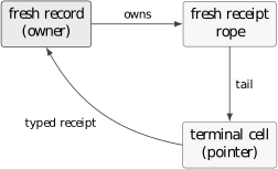
An earlier internal version of the allocation model (numbered PC-83 in the project’s records) allowed a fresh field to name only an already constructed fresh slot, and its finite checker imposed the same topological order. Figure 5 is therefore a genuine proof defect in that version: the claimed source transition was outside its own model. The rest of this section is the repair, stated for arbitrary bounded record programs.
9.2 Bounded simultaneous record transducers
Definition 9.1 (Simultaneous record batch). Fix constants (roots), (fresh slots), (pointer fields per slot), and (old dereference radius), together with finite control, tag, and payload alphabets. A transition may inspect tags and payloads reached within old logical field dereferences from its roots. From that old observation it chooses the next control and one finite batch of at most records. Each fresh field and next root targets missing, a bounded old address, or any active slot of the same batch. No fresh slot is inspected while the plan is selected, and control does not branch on physical pointer identity.
The last clause permits self, forward, and mutual fresh references. The batch is a finite labelled graph specified all at once. Three small batches show what is allowed: a self-loop (one slot pointing to itself), a forward reference (slot pointing to slot ), and a mutual cycle (slots and pointing to each other).
Theorem 9.2 (Simultaneous-batch compiler; fixed virtual initialization). Every bounded simultaneous record transducer with parameters , one fixed finite immutable pointer-closed initial graph, and plans determined by finite control, the input letter and bounded labelled rooted unfoldings has an exact letter-synchronous native scaffolding-automaton implementation of degree and observation/update distance at most . Physical pointer identity is not an observable test; fixed initial records are virtual finite decoder data.
Proof. Strategy. Pack the whole batch into one node, use ports for fields, use with a slot tag for every fresh target, and check that decoding is exact.
The fixed initial graph is stored in a finite decoder table. An initialization flag supplies time-zero roots and acceptance; virtual records use no dynamic fresh slot. Pointer closure prevents a path entering that table from returning to later dynamic storage. The first input transition emits only its ordinary bounded dynamic batch, as in the companion Draft 5 compiler correction.
One physical scaffold node represents the whole logical batch. Its finite label records the active mask; every active tag and payload; and, for every root and field, the finite target-slot tag.
Ports represent roots. Port represents field of logical slot . A decoded pointer is a pair of a physical historical node and a slot. An old logical address beginning at root and following fields , , compiles to the physical word where each next slot is read from the finite target tag at the preceding edge. The observed depth- neighborhood contains this information.
Use a missing descriptor for missing, the compiled word for an old target, and physical for every fresh target. In the last case the new label supplies the requested target slot.
Assume the old physical heap decodes correctly. Induction along a logical old address proves that its physical word reaches the same old pointer. Missing decodes immediately. A fresh descriptor reaches the node currently being appended and its tag selects exactly the requested fresh slot. Applying these three cases to every root and field makes the decoded new finite adjacency table identical to the source batch, including all cycles. This is equality of finite labelled graphs; no recursive graph unfolding or fixed point is needed. Run induction gives exact simulation. All alphabets and plan branches are finite, proving the stated degree and distance bounds. ◻
Remark 40 (Where the cycle lives). There is no contradiction with Theorem 4.1. The physical scaffold still has only backward edges and self-loops. A logical record pointer is the larger coordinate , not the physical node alone. Following a physical edge keeps fixed while its finite edge tag changes the logical slot from to . An arbitrary finite cycle in the decoded fresh batch is therefore represented by one physical self-loop together with finite slot dynamics. The coordinate realization has moved cyclicity from physical time into the finite decoder state.
9.3 Staging a strict persistent sequence
The compiler solves the target representation problem but not the source evaluation problem. A cycle is safe only if the program can choose its allocation skeleton without following the fresh feedback edge. A data structure is persistent when old versions survive updates [6, §1], and purely functional in Kaplan and Tarjan’s strict sense when built only from the LISP primitives , , (pair construction and projection), with memoization excluded [11, p. 578, footnote 1].
Theorem 9.4 (Opaque-element staging). Let a strict purely functional sequence operation:
use only finite constructor tests and a worst-case bounded number of fixed-arity constructor, projection, and pointer steps;
treat elements of its base type as opaque atoms, with no equality, hashing, pattern match, identity test, or traversal through a base element, while permitting inspection of the representation’s own pairs, buffers, and recursive child structures; and
return a fixed finite tuple of roots and removed elements.
For fixed old roots and symbolic new elements, its control branch and fresh structural allocation graph are determined independently of the symbolic values. If one symbol denotes a fresh owner that stores a resulting sequence root, the owner and structural graph form one bounded simultaneous batch and compile by Theorem 9.2.
Proof. Run the bounded operation with distinct symbols in place of new elements. Induct over its bounded primitive steps. A constructor test or projection reads only an old structural record or an earlier fresh structural record. Element opacity prevents the control path from following or branching on a symbol. A constructor step adds one fixed-arity structural record whose fields are old pointers, earlier structural pointers, or symbolic elements. Thus the branch and an acyclic bounded structural allocation graph are fixed before element substitution.
Add the fresh owner slot and replace its symbol by a pointer to that slot. The substitution can create a cycle from the owner through the sequence structure and back through an opaque element field, but it cannot change the selected branch or work bound. Theorem 9.2 represents every edge of the resulting finite graph using old paths, missing, or plus a slot tag. ◻
Kaplan and Tarjan’s Theorem 5.1 gives worst-case constant-time push, pop, inject, and catenation for regular catenable steques in their strict purely functional model [11, p. 592]. It does not itself state the stronger conjunction needed by Theorem 9.4: a concrete finite constructor program, base-element opacity, a uniform fresh-allocation bound, and a uniform old-address-depth bound. Those are separate applicability obligations, not consequences silently imported from the asymptotic theorem.
9.4 The conditional application
Proposition 9.5 (Feedback programs compile). Let a persistent program, at each input letter, start from a fixed number of roots and perform a fixed finite composition of strict purely functional sequence operations satisfying the hypotheses of Theorem 9.4 on opaque pointer elements. In addition it may create a bounded number of fresh fixed-arity records whose layouts are determined by the same old observation and whose fields target old records, resulting sequence roots, or records in that fresh finite batch. At most one designated fresh owner’s pointer is stored as a base-type element of those sequences. Suppose the complete per-letter computation, including those sequence operations, follows old logical fields only within some fixed dereference radius . Then the program is a bounded simultaneous record transducer, and it has an exact letter-synchronous implementation by a finite scaffolding automaton of degree and distance at most for suitable finite .
Proof. By Theorem 9.4, each sequence operation, run with the fresh owner’s pointer replaced by a symbol, has a control branch and an acyclic structural allocation graph determined by old structure alone; a fixed finite composition of such operations therefore allocates a bounded acyclic skeleton and reads a bounded number of old fields. Adding the bounded fixed-arity records, including the designated owner when present, and substituting that owner for its symbolic base element yields one finite batch of bounded size. Its fields target only bounded old addresses, structural sequence roots, or active fresh slots. This is a transition of Definition 9.1 with the total allocation bound and the maximal record arity. Theorem 9.2 compiles it. ◻
Example 9.6 (the conditional direct even-palindrome client). The sequence API is empty, single, uncons, and catenation; inject is catenation with a singleton. Both catenation operands can be unbounded. The generic compiler is independent of this application. In the companion's current Draft 5, Theorem 12.2 and Corollary 12.3 assume the complete Section 11.1 contract: list semantics, persistence, opacity, finite source-record signatures and inspected data, uniformly bounded strict evaluation and field selection, complete old/fresh pointer origins, and no escaping temporary control values. Under that premise, receipt closure, staging and whole-client normalization give a native scaffold and then a PEG for , using reversal invariance. Appendix D remains informal implementation evidence and Needs work; it does not certify the complete contract. Numerical radius and distance remain withdrawn. The earlier T89/T90 transfer paper [10] retains its separate route and status.
What this does and does not say. Proposition 9.5 repairs the allocation seam in general. It does not assert that any particular program satisfies its hypotheses; that is a separate proof obligation for each application.
10 Open boundaries
The proved general object is strong-trace equivalence. The broader program begins where final observation forgets that trace.
Unrestricted final presentation. Determine whether a finite graph-local move family presents final behavioral equivalence at all fixed degrees and distances. In plain terms: is there, for every , a finite list of local rewrites connecting any two histories with the same final figure? Dedicated relation exchange may be a primitive or may be derivable by refactoring older rows.
Elementary higher coherence. The strong normalizer gives one object normal form, garbage fibres are cubical, and unary carrier chambers form distributive lattices. A finite set of cells presenting all mixed derivations—elementary identities between sequences of moves of all three kinds—is open.
Support handoff. A temporal slide can transfer one visible label obligation across a causal cut. Classify its interactions (critical pairs) with detours and absorption.
Navigation monoids. Characterize which finitely generated submonoids of the regressive chain monoid occur at fixed degree, distance, and uniform finite control.
Functional sharing versus branching. Separate ordinary immutable record DAGs from unrestricted scaffold navigation first at the dynamic or observational level, before seeking a language separation.
Comparator theorem. Construct the precise structure-preserving translation, if one exists, from the guarded causal presentation calculus to an established cyclic term-graph rewriting system [2] or to the categorical presentation of term graphs [8]. Novelty should be judged only after that comparison.
11 Assurance, provenance, and nonclaims
The theorem proofs in this paper are ordinary written mathematical proofs. Executable enumeration is used separately to find counterexamples and corroborate finite instances. No proof assistant is used as a stronger label for the mathematics here.
| Layer | What it establishes |
|---|---|
| Written proof | the stated theorem for all objects satisfying its hypotheses |
| Finite audit | exact behavior over one explicitly bounded search domain |
| Source audit | the external theorem or model says what the paper attributes to it |
| Specialist review | documented external specialist critique has examined correctness and positioning; this row does not assert that such review has occurred |
| Novelty review | the contribution has been compared broadly enough to support priority language |
The public package includes a theorem inventory, proof audit, source audit, finite audit code, and exact output. The finite audits enumerate bounded histories (for instance all unary distance-one histories up to a fixed length), search for split fibres, and check the displayed normalizers; their counts are recorded in the package. They corroborate; they are not the proofs.
What is inherited.
Coalgebraic minimization and functional bisimulation [15]; ordinary acyclic-state merging [5]; general cyclic term-graph fold/unfold and confluence [2]; the scaffold model and its PEG correspondence [12]; strict real-time catenable steques [11]. No unrestricted final-equivalence or finite higher-coherence theorem is claimed; the palindrome example is not a theorem of this paper; and at this review stage no novelty claim is made.
What the viewpoint contributed.
The separation in Figure 1 repeatedly changed the mathematical target: treating physical endpoint equality and behavioral equality as different observations produced the unfolding quotient and exposed pure aliases as presentation data; retaining every prefix figure produced a right-stable strong congruence and the detour/unroll normal form; forgetting prefixes only afterward exposed temporal carrier motion and causal support as final-observation coordinates; treating a receipt as a typed coordinate rather than a semantic existence assertion exposed the same-step allocation cycle; and moving from topological allocation to a simultaneous coordinate realization turned that apparent impossibility into ordinary feedback with finite slot state. Each arrow of is a theorem obligation. In particular, a universal graph embedding is not automatically a bounded coordinate realization, and final language equality does not imply equality of causal histories.
Provenance and AI assistance.
The arguments were developed in FPRD Lab, an AI-assisted research project. The mathematics is the author’s responsibility; AI systems drafted and checked text and code under the author’s direction, and an adversarial pass found the allocation defect of Section 9 in an internal draft before publication. Load-bearing external statements are cited with locators and source scope. A later source audit found that the Kaplan–Tarjan theorem had been asked to carry an unstated implementation bridge; the correction above keeps that bridge open rather than attributing it to the source. This paper and the companion paper [9] were developed contemporaneously; neither treats the other as established, and every theorem of this paper is proved from its own text and the cited literature.
12 Conclusion
Persistent scaffold computation has an intrinsic algebra before one asks which language a machine recognizes. Its generated behavioral figures are ordered residual systems. Guarded static folds collapse equivalent presentations; chronological detours and one -unroll lift that collapse to a convergent presentation of full strong traces. Final observation then reveals a second layer—causal support, garbage cubes, temporal carriers, and cross-cut sewing—whose unrestricted presentation remains open.
The receipt knot explains why this distinction matters computationally. The semantic record exists, but a topologically ordered presentation cannot build it. In a simultaneous scaffold coordinate system the same cycle is a finite batch of edges with slot tags. That change of representation repairs the generic same-step allocation seam. The companion uses that compiler only under its complete Section 11.1 sequence contract; the implementation evidence leaves that premise open. More importantly, the generic construction exhibits the general principle: complexity can move between semantic structure, presentation dynamics, and observation without disappearing.
A Move and preservation table
| Move | Local action | Guaranteed preservation |
|---|---|---|
| endpoint detour | rename one bounded word with the same physical endpoint | every prefix figure and every common suffix |
| / absorption, unroll | replace an old recursive carrier by fresh | every prefix figure and every common suffix |
| garbage change | change data outside one source-certified replay support | final rooted concrete scaffold |
| temporal slide | move a unary residual carrier across one adjacent time cut | final behavioral figure |
| routing crossing | reassign demanded router slots injectively and transport selectors | final concrete consumer endpoints |
| relation exchange | exchange two dedicated factorizations with one old endpoint | final concrete consumer endpoints |
B The central implication map
References
[1] Federico Ardila, Megan Owen, and Seth Sullivant. Geodesics in CAT(0) cubical complexes. Advances in Applied Mathematics, 48(1):142–163, 2012. https://doi.org/10.1016/j.aam.2011.06.004.
[2] Zena M. Ariola and Jan Willem Klop. Equational term graph rewriting. Fundamenta Informaticae, 26(3–4):207–240, 1996. https://doi.org/10.3233/FI-1996-263401. Earlier version: CWI report CS-R9552, 1995 (the version inspected).
[3] Janusz A. Brzozowski. Derivatives of regular expressions. Journal of the ACM, 11(4):481–494, 1964. https://doi.org/10.1145/321239.321249.
Source[4] Noam Chomsky and Marcel-Paul Schützenberger. The algebraic theory of context-free languages. In P. Braffort and D. Hirschberg, editors, Computer Programming and Formal Systems, pages 118–161. North-Holland, 1963.
[5] Jan Daciuk, Stoyan Mihov, Bruce W. Watson, and Richard E. Watson. Incremental construction of minimal acyclic finite-state automata. Computational Linguistics, 26(1):3–16, 2000. https://aclanthology.org/J00-1002/.
[6] James R. Driscoll, Neil Sarnak, Daniel D. Sleator, and Robert E. Tarjan. Making data structures persistent. Journal of Computer and System Sciences, 38(1):86–124, 1989. https://doi.org/10.1016/0022-0000(89)90034-2.
[7] Bryan Ford. Parsing expression grammars: A recognition-based syntactic foundation. In Proceedings of POPL 2004, pages 111–122. ACM, 2004. https://doi.org/10.1145/964001.964011.
[8] Tobias Fritz and Wendong Liang. Free gs-monoidal categories and free Markov categories. Applied Categorical Structures, 31(2):21, 2023. https://doi.org/10.1007/s10485-023-09717-0. arXiv:2204.02284.
[9] Joshua Gay. Persistent receipts and simultaneous records: a direct scaffold for even palindromes. FPRD Lab review paper, Draft 5, 21 September 2026. FPRD reading edition.
[10] Joshua Gay. Real-time multitape languages transfer to parsing expression grammars. FPRD Lab review paper, released 5 August 2026. FPRD reading edition.
[11] Haim Kaplan and Robert E. Tarjan. Purely functional, real-time deques with catenation. Journal of the ACM, 46(5):577–603, 1999. https://doi.org/10.1145/324133.324139.
[12] Bruno Loff, Nelma Moreira, and Rogério Reis. The computational power of parsing expression grammars. Journal of Computer and System Sciences, 111:1–21, 2020. https://doi.org/10.1016/j.jcss.2020.01.001. Expanded preprint arXiv:1902.08272v2 (2020); definition and theorem numbers in this paper follow the preprint.
[13] Anil Nerode. Linear automaton transformations. Proceedings of the American Mathematical Society, 9(4):541–544, 1958. https://doi.org/10.1090/S0002-9939-1958-0135681-9.
[14] Jean-Éric Pin. Mathematical Foundations of Automata Theory. Lecture notes, MPRI; author-hosted, version retrieved 22 August 2026. https://www.irif.fr/~jep/PDF/MPRI/MPRI.pdf.
[15] Jan J. M. M. Rutten. Universal coalgebra: a theory of systems. Theoretical Computer Science, 249(1):3–80, 2000. https://doi.org/10.1016/S0304-3975(00)00056-6.
Reading-edition notes
This expanded web edition preserves the mathematical statements and proofs of the earlier publication, with the corrections recorded in the publication audit. The linked PDF is the retained corrected Draft 4 edition. This web edition aligns the generic compiler and Example 9.6 with the reviewed fixed virtual initialization and the companion Draft 5 conditional application; it does not rewrite the earlier PDF or claim new proof validation. Historical computational and formal-verification reports retain their original scope; they have not all been rerun for this revision.
Afterword: FPRD Lab’s contribution
9 September 2026 · Methodological and contribution addendum. The paper’s mathematical scope and review status remain as stated in the paper.
The Lab’s approach
FPRD means Finitely Presented Recognition Dynamics. Its starting point is to distinguish a finite description, the possibly infinite process it generates, and what an observer can learn from that process. Equal answers need not come from equal internal structures. Conversely, an infinite state space may have a short, exact description and useful coordinates; failure to compress it into finitely many states need not end the investigation.
A small example: balanced parentheses
The grammar S → (S)S | ε presents the language of
balanced parentheses. To recognize a prefix, keep the number of
unmatched opening parentheses, or a failure state if a closing
parenthesis arrived too early. An opening parenthesis increments the
count. A closing parenthesis decrements a positive count; at zero it
enters failure. Failure persists. At the end, accept exactly when the
count is zero.
The prefixes ( and ()( leave the same
future task: any suffix that completes one completes the other. The
prefix (( leaves a different task: ) completes
the first two prefixes but not this one. These future tasks are
residuals. There are infinitely many counts, yet a
finite set of update rules generates their dynamics. This is a classical
automata example, not a discovery of FPRD Lab. It illustrates the
research question: which coordinates preserve all relevant futures, and
what does updating or reading those coordinates cost?
From viewpoint to proof
In practice, the Lab fixes the observable and the allowed operations, compares presentations of the same problem, and seeks an exact translation or invariant. A failed shortcut is useful when a counterexample identifies the missing coordinate or hypothesis. Small computations test particular uncertainties; a proof must explain why the result holds beyond those tests. Costs, relation sides, boundary conditions, and the direction of each translation remain explicit.
AI-assisted exploration, source comparison, executable checks, and adversarial reconstruction support this work. Their agreement is not automatically independent evidence: shared assumptions must be exposed. A formal development certifies its stated formal theorem, not every interpretation attached to it. Each paper retains its own evidence and review status.
The approach is most useful when a poor representation hides a reusable construction, a compatibility condition, or a sharp obstruction. Outside recognition theory, it can guide the search for a structural reformulation without producing a literal residual dynamical system. The account below distinguishes that methodological influence from the ingredients of the proof.
FPRD’s contribution to this paper
This paper turns the distinction between presentation and observation into its main mathematical object. A row word, the physical history it builds, the behavior visible after every prefix, the final rooted behavior, and the final acceptance answer retain progressively different information. The Lab asked which transformations preserve each one.
That separation produced two different problems. Preserving the whole sequence of prefix observations leads to a strong-trace congruence and a guarded detour/unroll normal form. Preserving only the final observation permits additional changes in when useful records are carried. The paper analyzes those changes without promoting final agreement to agreement under every future context.
Its causal-support construction also distinguishes an unreachable node from an irrelevant construction step. A final edge can depend on an old edge that was copied when the final graph was built. A valid garbage change must respect that replay dependency. Tracking those dependencies supplies the sewing argument and, in the unary case, a concrete geometry of carrier placements.
The feedback analysis exposed a second representation error: an allocation model requiring fresh records to be built in topological order could not express a cycle required by a receipt. Simultaneous finite slots and the scaffold’s existing SELF descriptor repair that interface. The paper proves the compiler principle separately from its companion’s palindrome application. The companion's current Draft 5 keeps the direct consequence conditional on its complete Section 11.1 sequence contract. Whole-client normalization is a theorem under its hypotheses; the concrete implementation remains informal evidence with open source-contract obligations, and numerical radius/distance remain withdrawn.
Inherited ingredients and the boundary of the contribution
Loff, Moreira, and Reis supply the machine model. Coalgebraic minimization, bisimulation, persistent data structures, and cyclic term-graph rewriting are established sources, credited in the paper. The Lab’s contribution is the source-sensitive causal presentation calculus and its exact preservation theorems, including the distinction between replay support and final reachability.
The finite history checks helped locate failures; the causal arguments establish the general statements. No complete proof-assistant formalization is claimed. The unrestricted final-equivalence calculus remains open, and comparison with existing term-graph presentations remains a separate obligation. A normal form for a semantic object is not automatically a bounded online procedure for finding it.
Where to inspect the contribution: the paper, Sections 3–9 and 11, including the move-preservation table and the repaired allocation model.