One new node can preserve several changing stacks

A stack is a sequence whose first item can be pushed or popped. A persistent stack keeps old versions available: pushing an item creates a new head pointing to the old stack, while popping selects an already existing tail. Nothing has to erase the old version.

The obstacle in a scaffolding automaton seems to be its pace. It may create exactly one physical graph node for each incoming symbol. What if the simulated machine changes several stacks during that symbol?

The construction makes one physical node represent a tuple of logical stack heads. Its label stores one top symbol per stack. Its named edges store the corresponding tails. The number of stacks and the symbol alphabet are fixed in advance, so the tuple label still belongs to a finite alphabet. There is no need to allocate a separate physical node for every logical head.

For example, suppose the two stacks are ab and x, with their tops written first. The next symbol asks us to pop the first and push y onto the second. The result should be b and yx. The new node stores the label pair (b,y). Its first edge skips to the first stack’s old second tail; its second edge points to the old physical top, whose second component begins with x. Following the first named port decodes one stack, and following the second decodes the other. The same physical node can therefore be an old record for both stacks without confusing their meanings.

Only a bounded neighborhood is needed. Push refers to the old top; keep refers to one old tail; pop reads the old tail’s head and refers to its tail. Two edge steps suffice. The proof below also treats empty stacks, because an empty pop must not expose a stale symbol from an older version.

This gives a route from ordinary work tapes to parsing expression grammars. Represent a tape by the cells to the left of its head, the currently scanned symbol, and the cells to its right. The two sides are stacks. A head move pushes the symbol just written onto one side and pops the next scanned symbol from the other. A fixed number of tapes therefore becomes a fixed number of persistent stacks, all updated together.

Loff, Moreira, and Reis’s characterization then says that a scaffold for a language gives a PEG for its reversal. This direction matters: the construction does not assert that every real-time language itself has a PEG. Even palindromes are a useful application because reversing an even palindrome leaves the same word, so the orientation disappears in that case.

The real-time premise is exact. A machine that spends a long time after the last input symbol is outside it. So is a bound that averages cheap and expensive steps while allowing an arbitrarily expensive individual step. The article proves the machine-to-scaffold transfer directly; its palindrome application uses the classical recognizer and the source-model correspondence developed in Section 6 and Appendix C.

The main mechanism is in the update table of Section 3. The tape calculation in Section 4 explains why it applies to ordinary machines. The final part identifies which conclusions also use the historical real-time palindrome results. This positive construction complements the late-query obstruction: persistence can make a great deal of old information locally available, but it cannot make every future query cheap.

1 Introduction

Parsing expression grammars (PEGs), introduced by Ford [1], are recognition-based grammars whose ordered choice operator gives them behavior quite different from context-free grammars. Loff, Moreira, and Reis introduced scaffolding automata and proved that they characterize PEG languages up to reversal [4, Theorem 16]. They also proposed the following test of the formalism’s power: $$\mathsf{EPAL}_2 :=\{ww^R:w\in\{0,1\}^*\},$$ the language of even-length binary palindromes. Their Conjecture 7 states that $\mathsf{EPAL}_2\notin\mathsf{PEG}$.

The key observation of this paper is that one scaffold node can act as a persistent cons cell for several logical stacks at once. Its finite label is a tuple of stack-top symbols, and its named backward ports point independently to the persistent predecessor of each stack. Thus one physical append operation can perform a fixed tuple of logical memory updates.

This yields the main transfer theorem.

Together with the online lower bound already proved by Loff–Moreira–Reis, the transfer gives a proper class containment: $$\mathsf{rev}(\mathsf{RT\text{-}MTTM})\subsetneq\mathsf{PEG}.$$

The proof has two parts. First, a fixed collection of stacks, each performing one push, keep, or pop operation per input symbol, is simulated letter-for-letter by a distance-two scaffolding automaton. Second, the usual two-stack zipper represents each Turing tape. The resulting scaffold has degree $2m$ for an $m$-tape machine.

The proof path is therefore $$\begin{aligned} \boxed{\text{strict real-time multitape machine}} &\longrightarrow \boxed{2m\text{ persistent stacks}}\\ &\longrightarrow \boxed{\text{degree-}2m\text{ scaffold}}\\ &\longrightarrow \boxed{\text{PEG for the reverse}}. \end{aligned}$$ The construction is effective, although the generic PEG obtained by direct expansion is not expected to be compact or human-readable.

Slisenko constructs a real-time multitape palindrome recognizer [6]. Leong and Seiferas give an ordinary single-head multitape implementation [3]. A parity bit restricts the recognizer to even lengths. Since $(\mathsf{EPAL}_2)^R=\mathsf{EPAL}_2$, theorem 1.1 gives the announced consequence.

The historical direction is worth noting. Loff, Moreira, and Reis explicitly investigated whether reversals of PEG languages admit efficient online Turing-machine recognition and refuted that proposed containment [4, Section 5.3]. The construction here travels from strict real-time machines to scaffolding automata and then applies their characterization.

2 Models and conventions

For a word $x=x_1\cdots x_n$, write $x^R=x_n\cdots x_1$, and for a language $L$, write $L^R=\{x^R:x\in L\}$. For a language class $\mathcal C$, define $$\operatorname{rev}(\mathcal C)=\{L^R:L\in\mathcal C\}.$$ All alphabets and state sets below are finite. Throughout, $\mathsf{PEG}$ is Loff–Moreira–Reis’s class of ordinary total PEGs: the start expression must succeed while consuming the complete input. This is complete-match PEG semantics, not a prefix-acceptance variant [4, Definitions 1–4].

2.1 Scaffolding automata

We use the model of Loff, Moreira, and Reis [4, Definitions 10–15]. A scaffold of degree $d$ consists of a sequence of labelled nodes. Each node has $d$ named ports, and every port is either missing or points to a node no later than its source. The scaffold begins with an unlabelled base node.

On each input symbol, the automaton appends exactly one labelled node. Its transition sees the state and the depth-$k$ unfolding of the old top: a partial, labelled, $d$-ary tree that records labels along named port paths but not node identity. Each port of the new node may be left missing, may target the new node itself, or may target the endpoint of a port word of length at most $k$ starting at the old top. The fixed constants $d$ and $k$ are the degree and distance.

Acceptance depends on the finite control state immediately after the last input symbol. The characterization we use is:

This is the state duplication used without loss of generality in the sufficient direction of Loff–Moreira–Reis Theorem 16 [4, p. 23].

2.2 Strict real-time multitape machines

We use the letter-synchronous real-time convention of Rosenberg [5]: after each arriving input symbol, the machine performs exactly one transition and the resulting state reports the answer for the prefix then seen.

The input is an arriving symbol, not a preloaded input tape. In particular, the transition receives neither the total input length nor an end-of-input work interval.

3 Parallel persistent stacks

We first isolate the mechanism responsible for the transfer. Consider a deterministic finite-control machine with $s\geq 1$ stacks over a finite alphabet $A$. On every input step it reads the $s$ top symbols and performs one of $$\operatorname{push}(a),\qquad \operatorname{keep},\qquad \operatorname{pop}$$ on each stack. Popping an empty stack leaves it empty.

We construct a scaffolding automaton of degree $s$ and distance two. Reserve port $j$ for stack $j$, and take the scaffold alphabet to be $$\Gamma=(A\cup\{\bot\})^s.$$ For a scaffold node $v$, let $\lambda_j(v)$ denote component $j$ of its label and let $e_j(v)$ be its port-$j$ target. Adjoin a sentinel $\varnothing$ and set $$e_j(\varnothing)=\varnothing, \qquad \lambda_j(\varnothing)=\bot.$$ An unlabelled node also has component $\bot$. Following an invalid port path yields $\varnothing$, exactly as the missing-edge clause in Loff–Moreira–Reis Definition 13 requires.

The stack rooted at $v$ is decoded recursively by $$D_j(v)= \begin{cases} \varepsilon,&\lambda_j(v)=\bot,\\ a\,D_j(e_j(v)),&\lambda_j(v)=a\in A, \end{cases} \tag{1}$$ with $D_j(\varnothing)=\varepsilon$. The recursion terminates because the construction uses only strictly backward targets.

3.1 The update table

Let $v$ be the old scaffold top and $v^+$ the new one. Component $j$ of $v^+$ and port $j$ are selected as follows:

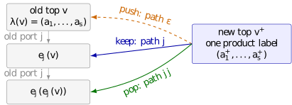
Every label read and every target named by this table occurs in the depth-two unfolding of $v$. The same newly appended node carries all $s$ component and port choices simultaneously.

The empty-stack case requires one invariant. Define $$\mathsf{CleanEmpty}(S) \quad\Longleftrightarrow\quad \forall v\in V\cup\{\varnothing\},j, \lambda_j(v)=\bot \Longrightarrow \lambda_j(e_j(v))=\bot. \tag{2}$$ Thus a node that terminates stack $j$ points, if anywhere, to another node that also terminates stack $j$. This prevents an empty pop from exposing a stale symbol through a historical port.

4 From work tapes to persistent stacks

Represent work tape $i$ by a zipper $$(L_i,c_i,R_i),$$ where $c_i$ is the scanned symbol, $L_i$ lists the cells strictly to the left of the head in nearest-first order, and $R_i$ lists the cells strictly to the right in nearest-first order. The scanned symbols $(c_1,\ldots,c_m)$ are stored in finite control. Blank cells beyond the finite lists are supplied by the fixed blank convention. Here $\sqcup$ is an ordinary tape-alphabet symbol; $\bot$ means that a finite stack has no next element and is not a tape symbol. Initially $L_i=R_i=\varepsilon$ and $c_i=\sqcup$ on every tape.

For extensional comparison with the source tape, define $$\operatorname{cell}_{L,c,R}(z)= \begin{cases} c,&z=0,\\ L_{-z},&z<0\text{ and that entry exists},\\ R_z,&z>0\text{ and that entry exists},\\ \sqcup,&\text{otherwise}. \end{cases} \tag{3}$$

Suppose the machine writes $b_i$ and then moves its $i$-th head. The zipper updates are: $$\begin{array}{rcl} \text{right:}& (L_i,c_i,R_i)&\mapsto (b_iL_i,\operatorname{head}_{\sqcup}(R_i),\operatorname{tail}(R_i)),\\[2mm] \text{left:}& (L_i,c_i,R_i)&\mapsto (\operatorname{tail}(L_i),\operatorname{head}_{\sqcup}(L_i),b_iR_i),\\[2mm] \text{stay:}& (L_i,c_i,R_i)&\mapsto (L_i,b_i,R_i). \end{array} \tag{4}$$ Consequently each ordinary tape transition performs at most one operation on each of the two stacks $L_i,R_i$. All $m$ tapes update in parallel.

5 The real-time transfer

6 Even-length palindromes

Let $$\mathsf{PAL}_2=\{x\in\{0,1\}^*:x=x^R\}.$$

The only external premise needed here is stated directly in the source model of definition 2.3. It is a classical imported theorem: the proof below audits the source-model correspondence, while the source theorem itself is not re-mechanized here.

7 Formal verification

The reviewed Lean 4 source snapshot is commit 20ef2ef5f14274e37ac0dd40af0f944ff34885ce ². The same source directory on the maintained branch is available here ³. It uses Lean 4.30.0 without Mathlib.

The principal endpoints are:

• realtime_transfer_tape_contents;

• scaffold_to_peg;

• revRT_multitape_subset_PEG; and

• epal2_inPEG_of_multitape_recognizer.

The last is the conditional EPAL implication: no palindrome recognizer is introduced as an axiom. Exhaustive finite carriers and bounded port paths produce a literal finite nonterminal type, and the grammar handles automata that use SELF. Searches over the source find no sorry, admit, declared axiom, unsafe, native_decide, or partial def. For all four principal endpoints listed above, #print axioms reports only propext, Classical.choice, and Quot.sound. The occurrence of Classical.choice comes from standard classical finite-carrier and transport constructions in the proof; it is not an added mathematical hypothesis about automata or languages.

As a separate implementation check, a literal interpreter of the published scaffold transition model was tested with a transferred four-stack middle-symbol machine. Exhaustive tests through length $14$, longer structured and random tests, and eight deliberately corrupted variants exercise the unfolding and port-word resolution independently of the Lean development.

8 Discussion

The transfer rests on a simple resource principle: the number of physical updates and the number of logical memory roots updated need not coincide. A scaffold node has a product label and a fixed tuple of named ports, so one append can advance every root in a fixed finite family. The two-stack zipper then converts local movement on each work tape into exactly this form.

This also explains why an explicit midpoint is unnecessary in the palindrome application. The scaffolding automaton does not discover the midpoint by a single stack turn. It simulates the distributed schedule already present in the classical real-time recognizer.

The degree is a fixed parameter of the scaffolding automaton, not a universal bound on the model. An $m$-tape realization uses degree $2m$ and distance two. No pointer-identity test is needed: the transition reads only labels along named paths in the published tree unfolding.

9 Conclusion

A fixed tuple of persistent stack roots can be updated by one appended scaffold node. Through the ordinary two-stack representation of a Turing tape, this gives an exact letter-synchronous simulation of strict real-time multitape computation. The Loff–Moreira–Reis characterization therefore places the reversal of every such language in $\mathsf{PEG}$. Applied to the classical real-time palindrome recognizer, the transfer yields a PEG for even-length binary palindromes.

The assurance boundary is exact. Lean machine-checks the compiler equality $L(A_M)=L(M)$, the sufficient scaffold-to-PEG construction, the strict-real-time containment, and the implication from an exact strict real-time multitape EPAL recognizer to $\mathsf{EPAL}_2\in\mathsf{PEG}$. The Loff–Moreira–Reis, Slisenko, Leong–Seiferas, and fixed-rate speedup results supply the properness and recognizer premises; they were checked against the cited classical statements but not mechanized. Thus the EPAL and proper-containment conclusions are established, while the classical source layer is not re-mechanized in this repository. The enormous generic PEG is not expanded here.

A The persistent update, literally

This appendix expands the compact proof of lemma 3.1. The sentinel conventions make every expression in the update table total: $$e_j(\varnothing)=\varnothing, \qquad \lambda_j(\varnothing)=\bot, \qquad D_j(\varnothing)=\varepsilon.$$ If a port is missing, or a port word first becomes invalid, all remaining steps stay at $\varnothing$. Thus the expressions $e_j(v)$ and $e_j(e_j(v))$ have literal meanings even at the boundary.

Fix $j$. For a push, the new node has head $a$ and tail root $v$, so $$D_j(v^+)=aD_j(v).$$ For keep, if $\lambda_j(v)=a$, the new node has head $a$ and tail $e_j(v)$, hence reproduces $D_j(v)$. If $\lambda_j(v)=\bot$, both old and new decodings are empty. For pop, if $D_j(v)=aD_j(e_j(v))$, then the new head is $\lambda_j(e_j(v))$, its new tail is $e_j(e_j(v))$, and therefore $$D_j(v^+)=D_j(e_j(v)).$$ If $D_j(v)=\varepsilon$, $\mathsf{CleanEmpty}$ gives $\lambda_j(e_j(v))=\bot$, including when $e_j(v)=\varnothing$, so the pop remains empty. Push cannot create an empty component. Keep inherits the clean-empty implication from $v$, and pop inherits it from $e_j(v)$. All named targets are at or below the old top, so they are strictly behind the newly appended node.

Here is the simultaneous two-stack case in one line. Suppose $$D_1(v)=a\alpha, \qquad D_2(v)=b\beta.$$ Push $x$ on stack 1 and pop stack 2. The single new node has components $x$ and $\lambda_2(e_2(v))$; its first port names $v$, while its second names $e_2(e_2(v))$. Consequently $$\bigl(D_1(v^+),D_2(v^+)\bigr) =\bigl(xa\alpha,\beta\bigr).$$ The two logical updates are simultaneous because both components and both ports belong to the same appended node. If $\beta=\varepsilon$, the sentinel and $\mathsf{CleanEmpty}$ calculation above makes the second result empty.

B Extensional tape reconstruction

Let $Z=(L,c,R)$ be a zipper and let $b$ be the symbol written before the head moves. Define the tape after the write but before the move by $$\operatorname{written}_{Z,b}(z)= \begin{cases} b,&z=0,\\ \operatorname{cell}_{L,c,R}(z),&z\ne0. \end{cases}$$ If $Z_{\rightarrow}$, $Z_{\leftarrow}$, and $Z_{\circ}$ are the three zippers in (4), then for every $z\in\mathbb Z$, $$\begin{aligned} \operatorname{cell}_{Z_{\rightarrow}}(z) &=\operatorname{written}_{Z,b}(z+1),\\ \operatorname{cell}_{Z_{\leftarrow}}(z) &=\operatorname{written}_{Z,b}(z-1),\\ \operatorname{cell}_{Z_{\circ}}(z) &=\operatorname{written}_{Z,b}(z). \end{aligned}$$

For the right-move equation, $z=-1$ reads the newly pushed head of $bL$, hence $b$; $z=0$ reads $\operatorname{head}_{\sqcup}(R)$; positive offsets read the remaining tail of $R$; and offsets below $-1$ read the old entries of $L$. These are exactly the four cases of the right-hand side. The left equation is the mirror image, and stay changes only offset zero. The default $\sqcup$ in $\operatorname{head}_{\sqcup}$ and in (3) proves the equations even when either finite list is exhausted.

Initially $L=R=\varepsilon$ and $c=\sqcup$, so the reconstruction is blank at every integer offset. Induction on input length now maintains the following invariant for each work tape: the source control state and scanned symbol agree with the compiled control, and the source cell at every head-relative integer offset equals the cell reconstructed from the two decoded persistent stacks. This is the exact invariant asserted by theorem 4.2 and by the Lean theorem realtime_transfer_tape_contents.

C Classical palindrome interface audit

This appendix records how the classical statements discharge every clause of theorem 6.1. A longer source-audit note, including the rejected attempt to reconstruct the final theorem from positive-report sublemmas alone, is public with the paper. ⁴

The remaining source pins are Slisenko’s reporting conditions on p. 132 and Proposition 4.4 on p. 134, and Leong–Seiferas Theorems 3.1 and 3.5 and Corollary 3.6 on pp. 170, 173, and 174. Leong–Seiferas supply the storage realization; palindrome correctness comes from Slisenko’s final theorem.

Same-prefix timing

Fix a prefix $u$ and regard $u$ itself as a legitimate finite input. Slisenko’s real-time theorem decides it at tick $|u|$. The deterministic machine has received exactly the same symbols and no endmarker, length advice, or preloaded suffix after $|u|$ ticks on inputs $u$ and $uv$. Its configuration is therefore identical in the two runs. Hence the report at each tick is the two-sided verdict for the prefix read through that tick. This argument uses the final recognition theorem; it does not infer rejection correctness from Slisenko’s positive-report propositions.

Fixed-round strictification

Consider a fixed deterministic streaming reporter whose round receives one symbol, performs at most $c$ controller or tape-unit commands, and returns a Boolean report for that same prefix. Pad every branch to $c$ program positions, retaining the arriving symbol, a program counter, branch results, and a done bit in finite control. Positions after completion are no-ops.

Instantiate the deterministic Leong–Seiferas simulator for each logical multihead unit, give different units disjoint finite tape families, and take the finite product of their controllers with the padded reporter. Corollary 3.6 supplies the fixed ordinary single-head simulations. The blank-tape initialization of Theorem 3.1 establishes the base configuration without a startup phase.

Choose one fixed speedup rate large enough for the padded schedule and every unit simulator. The no-time-loss normalization cited on Leong–Seiferas p. 167 compresses the product round into one conventional global transition over a fixed enlarged alphabet. A selected tape performs its prescribed write and move; every other tape rewrites its scanned symbol and stays. Put the report bit in the finite control.

After a prefix $x$, maintain simultaneously:

1. equality of the source and simulated controllers and logical unit states;

2. equality of every decoded tape content and logical head position;

3. a boundary program counter and exactly $|x|$ consumed symbols; and

4. equality of the finite-control report bit and the reporter’s answer for $x$.

Blank initialization proves the base case. The no-delay unit simulations, padding, and fixed-rate normalization prove one-round preservation, including data-dependent branches. Induction gives the same report after every prefix with no output lag or finishing computation. Fill unreachable transition-table entries arbitrarily to obtain a total transition function. If the historical convention omits an empty report, a fresh accepting initial state delegates its first-symbol transition to the old initial transition and is never re-entered. This proves exactly the strict interface in theorem 6.1.

References

Source[1] Bryan Ford. Parsing expression grammars: A recognition-based syntactic foundation. In Proceedings of POPL 2004, pages 111–122. ACM, 2004.
Source[2] Zvi Galil. Palindrome recognition in real time by a multitape Turing machine. Journal of Computer and System Sciences, 16(2):140–157, 1978.
Source[3] Benton L. Leong and Joel I. Seiferas. New real-time simulations of multihead tape units. Journal of the ACM, 28(1):166–180, 1981.
[4] Bruno Loff, Nelma Moreira, and Rogério Reis. The computational power of parsing expression grammars. Journal of Computer and System Sciences, 111:1–21, 2020. https://doi.org/10.1016/j.jcss.2020.01.001.
Source[5] Arnold L. Rosenberg. Real-time definable languages. Journal of the ACM, 14(4):645–662, 1967.
[6] A. O. Slisenko. A simplified proof of the real-time recognizability of palindromes on Turing machines. Zapiski Nauchnykh Seminarov LOMI, 68:123–139, 1977. English translation in Journal of Soviet Mathematics, 15:68–77, 1981. https://doi.org/10.1007/BF01404109.
Reading-edition notes
This expanded web edition preserves the mathematical statements and proofs of the earlier publication, with the corrections recorded in the publication audit. The PDF is the earlier edition. Historical computational and formal-verification reports retain their original scope; they have not all been rerun for this revision.
Afterword: FPRD Lab’s contribution
9 September 2026 · Methodological and contribution addendum. The paper’s mathematical scope and review status remain as stated in the paper.
The Lab’s approach
FPRD means Finitely Presented Recognition Dynamics. Its starting point is to distinguish a finite description, the possibly infinite process it generates, and what an observer can learn from that process. Equal answers need not come from equal internal structures. Conversely, an infinite state space may have a short, exact description and useful coordinates; failure to compress it into finitely many states need not end the investigation.
A small example: balanced parentheses
The grammar S → (S)S | ε presents the language of
balanced parentheses. To recognize a prefix, keep the number of
unmatched opening parentheses, or a failure state if a closing
parenthesis arrived too early. An opening parenthesis increments the
count. A closing parenthesis decrements a positive count; at zero it
enters failure. Failure persists. At the end, accept exactly when the
count is zero.
The prefixes ( and ()( leave the same
future task: any suffix that completes one completes the other. The
prefix (( leaves a different task: ) completes
the first two prefixes but not this one. These future tasks are
residuals. There are infinitely many counts, yet a
finite set of update rules generates their dynamics. This is a classical
automata example, not a discovery of FPRD Lab. It illustrates the
research question: which coordinates preserve all relevant futures, and
what does updating or reading those coordinates cost?
From viewpoint to proof
In practice, the Lab fixes the observable and the allowed operations, compares presentations of the same problem, and seeks an exact translation or invariant. A failed shortcut is useful when a counterexample identifies the missing coordinate or hypothesis. Small computations test particular uncertainties; a proof must explain why the result holds beyond those tests. Costs, relation sides, boundary conditions, and the direction of each translation remain explicit.
AI-assisted exploration, source comparison, executable checks, and adversarial reconstruction support this work. Their agreement is not automatically independent evidence: shared assumptions must be exposed. A formal development certifies its stated formal theorem, not every interpretation attached to it. Each paper retains its own evidence and review status.
The approach is most useful when a poor representation hides a reusable construction, a compatibility condition, or a sharp obstruction. Outside recognition theory, it can guide the search for a structural reformulation without producing a literal residual dynamical system. The account below distinguishes that methodological influence from the ingredients of the proof.
FPRD’s contribution to this paper
The key question was how much logical work one legal scaffold append can represent. Treating “one new physical node” as “one new logical cell” would impose a restriction that the source machine model does not require.
The Lab supplied an explicit coordinate representation: one node carries a finite tuple of stack-top symbols, with separately named ports for the corresponding persistent tails. Push, keep, and pop become bounded observations and port choices. A distance-two neighborhood suffices. The representation invariant also handles empty stacks, where a careless decoder could expose stale data.
The familiar two-stack representation of a work tape then becomes useful in this precise setting. Two persistent stacks per tape, together with the scanned symbol in finite control, translate each strict real-time global transition into one scaffold step. The substantive bridge is this letter-for-letter simulation with fixed resources, not the mere observation that tapes can be encoded as graphs.
The method also forced an interface audit at the other end. Applying a historical palindrome recognizer requires an answer for the prefix just read, fixed finite storage units, and no unbounded finishing computation. The paper spells out the source conventions and their normalization instead of treating every use of “real time” as interchangeable.
Inherited ingredients and the boundary of the contribution
Persistent stacks and the tape zipper are established constructions. Loff, Moreira, and Reis supply the exact scaffold/PEG characterization, including reversal. Slisenko supplies the real-time palindrome recognizer; Leong and Seiferas supply the ordinary single-head simulation used in the source-interface argument. The Lab’s contribution is the explicit bounded scaffold realization and the checked composition of these interfaces.
Consequently, the theorem transfers the reversal of a strict real-time multitape language to PEGs. Even palindromes are an application because that language is reversal invariant. The paper does not infer a compact practical PEG, a classification of PEG languages, or unrestricted simulation of machines with post-input work.
The paper records a Lean development and distinguishes it from the historical source audit. This afterword adds no formal-verification or review credit. It identifies where the presentation viewpoint became an actual machine construction.
Where to inspect the contribution: the paper, Sections 3–7 and Appendices A–C, especially the update table, tape reconstruction, and same-prefix timing argument.