Expanded reading edition · 5 September 2026
The string 0110 is an even palindrome: its second half
reverses its first. So are 00, 1001, and the
empty string. A grammar can describe all such words by repeatedly
wrapping the same symbol around a shorter palindrome. Recognizing the
words while input arrives is a different task. Before the input ends,
the recognizer is never told which position will be the middle.
A stack solves a related problem with a marked middle. Read the first half onto the stack, then compare incoming symbols with popped symbols after the marker. Removing the marker removes the moment at which that algorithm knows to switch roles. Keeping all plausible centers or walking back along many suffix links can take more work than one input step allows.
This article develops a direct persistent-graph construction. Its state describes the longest even-palindromic suffix of the input so far and the context to its left. A 10 September 2026 source-level audit now supplies an explicit fixed-layout resource certificate. A whole-client symbolic normalization theorem now closes the source-to-plan gap isolated by the end-to-end audit. The remaining weakest premise is the manual old-address certificate. Here is a short trace:
| Input so far | Longest even-palindromic suffix | Remaining prefix |
|---|---|---|
0 |
empty | 0 |
00 |
00 |
empty |
001 |
empty | 001 |
0011 |
11 |
00 |
00110 |
0110 |
0 |
001100 |
001100 |
empty |
At each step the complete prefix is an even palindrome exactly when the remaining prefix is empty. The mathematical challenge is to update this description with uniformly bounded local work, including at steps where the longest suffix changes dramatically.
The construction stores receipts: pointers to records whose correctness has already been established. A receipt is more than a length or an endpoint. It identifies the particular palindrome record needed by a future transition. A persistent sequence of these receipts can be shared by several contexts. The key recurrence proves that the shared cells carry the same receipts, even when the surrounding palindrome contexts differ. Equality of the underlying strings alone would not justify reusing the pointers.
There is a second challenge. A newly created palindrome record points to its new receipt sequence, and the last receipt in that sequence points back to the record. Both objects belong to the same input step. Ordinary sequential allocation cannot make both pointers point to already allocated objects.
The article resolves that issue by packing a fixed-size batch of logical records into one physical scaffold node. A finite slot number says which logical record is meant. An edge between two records in the same batch becomes a physical self-loop together with a slot tag. The physical graph obeys the scaffold rules even when the decoded batch contains a cycle. This compiler is proved separately from the palindrome recurrence, so its role can be inspected directly.
To keep the receipt-sequence operations bounded in the worst case, the construction starts from Kaplan–Tarjan’s purely functional catenable-sequence result. Section 11 separates that stated worst-case theorem from the stronger FPRD requirements: finite branching and allocation, bounded old-address access, and opacity of the complete stored cell. A later length-free source variant, constructor proof, allocation and exposure audits, fixed client layout, and max-plus composition now supply that stronger interface in an explicit abstract source-record model. This is not a literal OCaml runtime theorem or a correspondence proof with the separate Rocq implementation.
The persistent-stacks article takes a different route through classical real-time palindrome machines. Here the point is to expose how the palindrome information itself can be maintained in a scaffold. The running trace, the failed simpler representations, the receipt recurrence, and the batch compiler explain successive parts of that construction.
Guiding question. Can a device that adds only one bounded-local graph node per input letter recognize a language whose obvious description compares two unbounded halves?
Write \(w^R\) for the word \(w\) read backwards and \(\mathsf{EPAL}_2\) for the set of binary words of the form \(ww^R\): the even-length palindromes \(\epsilon\), \(00\), \(11\), \(0110\), \(1001\), \(001100\), and so on. As a generative object the language is as simple as they come: three rewriting rules produce it (Section 2.2). Loff, Moreira, and Reis (hereafter LMR) studied how much computational power the recognition-based grammars called parsing expression grammars have, and found both surprising positive examples and a natural negative conjecture [7, Conjecture 7, p. 10]:
The language of even-length palindromes has no PEG, i.e. \(P=\{ww^r\mid w\in\{0,1\}^*\}\notin\mathsf{PEG}\).
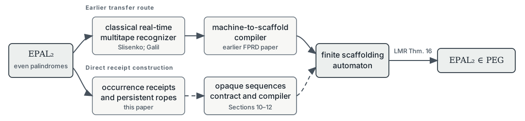
The intuition behind the conjecture is that a PEG cannot “find the middle” of its input. The conjecture is false. An earlier paper of this project [5] refuted it by compiling strict real-time multitape Turing machines into LMR’s scaffolding automata and invoking the classical theorem that palindromes are recognizable in real time by such a machine [9, 4]. That route proves membership but explains nothing about what a scaffold must remember to compare two halves.
This paper develops a second, direct route. The reader needs no Turing machine and no palindrome theorem: only words, finite graphs, and one inherited data structure. A later source-level certificate makes the data-structure interface explicit. Theorem 11.3 closes the source-to-plan gap isolated by the end-to-end audit. Figure 1 shows the two routes.
The lower route produces two separable results.
The direct application. The receipt construction gives a finite scaffolding automaton for \(\mathsf{EPAL}_2\) and then an ordinary PEG by LMR’s theorem. The source-resource constants belong to the abstract immutable-record model; their old-address proof remains manual rather than machine checked.
The reusable tool. Any one-step update that reads a bounded amount of old persistent structure and creates a bounded finite graph of fresh records—even a graph with cycles among the fresh records—can be performed by one scaffold node (Theorem 10.2). The palindrome construction is exactly what forces the cyclic case.
Section 2 defines everything the argument uses: words, context-free grammars, PEGs, scaffolding automata, persistence, and the mutable palindrome index that the scaffold cannot have. A reader who knows these objects may skim it, but should read Definition 2.6 and Theorem 2.7, whose exact form matters. Section 3 fixes three layers of description that the proof keeps separate. Section 4 follows one input word by hand. Part II proves the combinatorics of the longest even-palindromic suffix and turns it into operations on persistent ropes. Part III defines the compiler, proves it, and assembles the automaton. Part IV says what was proved, what is inherited, and what remains open.
Proofs state their strategy before their details. Every example says which of its features generalize. The compiler, conditional staging theorem, whole-client normalization theorem, and direct application are stated in this paper. Its external inputs are LMR’s Theorem 16 (sufficient direction) and Kaplan–Tarjan’s Theorem 5.1; the stronger finite-record interface used here is supplied by the later source-level certificate, not attributed to Kaplan–Tarjan.
An alphabet \(\Sigma\) is a finite set of letters; in this paper \(\Sigma=\{0,1\}\) unless stated otherwise. A word is a finite sequence of letters, \(\epsilon\) is the empty word, \(\Sigma^*\) is the set of all words, and \(|w|\) is the length of \(w\). Juxtaposition \(uv\) is concatenation. A language is any subset of \(\Sigma^*\). The reversal of \(w=c_1c_2\cdots c_n\) is \(w^R=c_n\cdots c_2c_1\); reversal of a language is \(L^R=\{w^R:w\in L\}\).
A word \(u\) is a suffix of \(w\) if \(w=xu\) for some \(x\), and a proper suffix if moreover \(u\ne w\); prefixes are defined symmetrically. The empty word is a proper suffix of every nonempty word. A palindrome is a word \(w\) with \(w=w^R\); an even palindrome is a palindrome of even length, equivalently a word of the form \(ww^R\). The empty word is an even palindrome. Thus \[\mathsf{EPAL}_2=\{ww^R:w\in\{0,1\}^*\}=\{\text{even palindromes over }\{0,1\}\},\] and \(\mathsf{EPAL}_2^R=\mathsf{EPAL}_2\) because reversing \(ww^R\) gives \(ww^R\) again.
When a palindrome \(P\) occurs as a suffix of a word \(S=CP\), the letter of \(C\) immediately to the left of that occurrence will matter constantly; we say the occurrence is preceded by that letter. The empty suffix of a nonempty word is preceded by the word’s last letter; the empty suffix of \(\epsilon\) is preceded by no letter.
A context-free grammar consists of a finite set of terminal symbols (our alphabet), a disjoint finite set of non-terminal symbols, a start non-terminal, and finitely many rewriting rules \(A\to\varphi\) in which \(A\) is one non-terminal and \(\varphi\) is a word over terminals and non-terminals [1, pp. 120–122]. A derivation starts from the start symbol and repeatedly replaces one occurrence of a non-terminal by the right-hand side of one of its rules, in any order, until only terminals remain. The language generated by the grammar is the set of terminal words obtained by some derivation.
Example 2.1 (even palindromes are context-free). With start symbol \(S\) and rules \[S\to 0S0,\qquad S\to 1S1,\qquad S\to\epsilon,\] the derivation \(S\Rightarrow 0S0\Rightarrow 01S10\Rightarrow 0110\) produces \(0110\), and in general the generated language is exactly \(\mathsf{EPAL}_2\): each rule adds one matching letter at each end, and every \(ww^R\) arises by choosing the letters of \(w\) in order. The reading is existential: a word belongs to the language if some sequence of choices produces it. Nothing in the definition says how a machine would discover those choices.
Parsing expression grammars, introduced by Ford [3, §3], use rule shapes that look like context-free rules but give them an operational meaning. We follow the formalization of LMR [7, Definitions 1–4], which is the one their theorem is stated for.
Definition 2.2 (parsing expressions and grammars). Fix disjoint finite sets \(\Sigma\) of terminals and \(\mathit{NT}\) of non-terminals. Parsing expressions are built from the atoms \(a\in\Sigma\), \(A\in\mathit{NT}\), \(\varepsilon\) (accept the empty word) and \(\mathsf{FAIL}\) by three constructions: sequence \(e_1e_2\), ordered choice \(e_1/e_2\), and the predicates \(!e\) and \(\&e\). A parsing expression grammar \(G\) assigns to each non-terminal \(A\) one expression \(R(A)\), written \(A\leftarrow R(A)\), and names a start non-terminal \(S\).
The meaning of an expression is a recognition procedure \(\operatorname{Rec}_G(e,x)\) that reads an input word \(x\) from the left and either fails or succeeds consuming a prefix \(x'\) of \(x\) [7, Definition 3 and Algorithm 1]:
\(\varepsilon\) succeeds consuming nothing; \(\mathsf{FAIL}\) fails; the terminal \(a\) succeeds consuming \(a\) if \(x\) begins with \(a\), and fails otherwise.
Sequence \(e_1e_2\): run \(e_1\) on \(x\); if it succeeds consuming \(y_1\), run \(e_2\) on the remainder; succeed consuming \(y_1y_2\) if both succeed, otherwise fail.
Ordered choice \(e_1/e_2\): run \(e_1\); if it succeeds, that is the answer; only if it fails is \(e_2\) run on the same input.
Predicates: \(!e\) succeeds consuming nothing if \(e\) fails, and fails if \(e\) succeeds; \(\&e\) succeeds consuming nothing if \(e\) succeeds.
A non-terminal \(A\) runs \(R(A)\).
The procedure is deterministic: at every point exactly one thing happens. It may loop forever (for example \(A\leftarrow A\)); a grammar is total if it never does. Following LMR, a total grammar recognizes the language \[L(G)=\{x\in\Sigma^*:\operatorname{Rec}_G(S,x)=x\},\] the words on which the start expression succeeds consuming the whole input, and \(\mathsf{PEG}\) is the class of languages recognized by total PEGs [7, Definition 4]. We call this complete-match recognition; it is the ordinary notion, not a variant.
Example 2.3 (order is semantic). Take \(S\leftarrow a/ab\) and the input \(ab\). The first alternative \(a\) succeeds consuming \(a\), so the choice commits to it: \(\operatorname{Rec}(S,ab)=a\ne ab\), and \(ab\notin L(G)\) although the second alternative would have consumed it. As a context-free grammar, \(S\to a\mid ab\) generates \(\{a,ab\}\). Ordered choice is not a parsing strategy for a context-free grammar; it changes the language. (Ford proves the corresponding algebraic fact: sequence distributes over ordered choice on one side only [3, p. 7].)
Example 2.4 (predicates see ahead without consuming). The expression \(!(0/1)\) succeeds exactly at the end of the input, consuming nothing, because it succeeds only where no letter can be read. Predicates let a PEG test a property of the remaining input and then parse it again. It is known that the non-context-free language \(\{a^nb^nc^n\}\) has a PEG [7, p. 3, citing Aho and Ullman], and LMR use predicates to recognize the palindromes of power-of-two length [7, Theorem 8, p. 10].
Example 2.1 shows \(\mathsf{EPAL}_2\) is context-free by three rules. One cannot read those rules as a PEG and hope: the choice \(S\leftarrow 0S0/1S1/\varepsilon\) commits to \(0S0\) whenever the input begins with \(0\), and then must find the matching closing \(0\) at a position it has no way to locate—a PEG consumes left to right and cannot “count to the middle”. That is the content of LMR’s conjecture. Conversely, PEGs recognize languages, such as \(\{a^nb^nc^n\}\) [7, p. 3], that no context-free grammar generates. Neither class contains the other by any syntactic argument; the comparison must go through a machine model. LMR supplied that model.
LMR’s machine builds a permanent graph. We give their definition [7, Definitions 10–15, pp. 14–16] in words first, then precisely, then with a picture.
In words: the machine reads one input letter at a time. Its memory is a growing directed graph whose nodes are numbered \(0,1,2,\ldots\) in the order of creation; node \(0\) is an unlabelled base, and every later node carries a label from a finite working alphabet and a fixed number \(d\) of ports (outgoing edges), each pointing to an older node, to the node itself, or to nothing. Old nodes are never changed. At each letter the machine looks only at the nodes within a fixed distance \(k\) of the most recently created node (the top), following ports; based on what it sees, on the letter, and on its finite control state, it creates one new node, chooses its label, and chooses where its ports point—necessarily among the nodes it just looked at, or the new node itself. After the last letter it accepts or rejects by its control state.
Definition 2.5 (scaffold). Let \(d\ge1\) and let \(\Gamma\) be a finite alphabet. A \((d,\Gamma)\)-scaffold with top \(t\) has nodes \(0,1,\ldots,t\), a label \(L(v)\in\Gamma\cup\{\varnothing\}\) for each node (\(L(0)=\varnothing\): the base is unlabelled), and for each node \(v\) and each port \(i\in\{0,\ldots,d-1\}\) a target \(e_v(i)\in\{0,\ldots,v\}\cup\{\varnothing\}\) (edges point backwards or to the node itself; \(\varnothing\) means the port is missing). A port word \(p=p_1\cdots p_m\) over \(\{0,\ldots,d-1\}\) is followed from a node by taking port \(p_1\), then port \(p_2\) of the node reached, and so on; it is valid from \(v\) if no missing port is met, and then it has an endpoint. The \(k\)-neighbourhood \(N_k(v)\) of a node is the labelled tree of depth \(k\) obtained by unfolding ports from \(v\): it records the label of every node reached by a port word of length at most \(k\), and where a port is missing. The tree records labels, not node numbers, so it does not reveal whether two port words reach the same node.
Definition 2.6 (scaffolding automaton). A scaffolding automaton is a tuple \(A=\langle\Sigma,d,\Gamma,k,Q,\delta,q_0,F\rangle\): an input alphabet \(\Sigma\), a degree \(d\ge1\), a working alphabet \(\Gamma\), a distance \(k\ge0\), a finite set of control states \(Q\) with initial state \(q_0\) and accepting states \(F\subseteq Q\), and a transition function \[\delta:\ Q\times\Sigma\times N_k(d,\Gamma)\longrightarrow Q\times\Gamma\times\bigl(\{0,\ldots,d-1\}^{\le k}\cup\{\mathsf{SELF},\varnothing\}\bigr)^d ,\] where \(N_k(d,\Gamma)\) is the set of possible \(k\)-neighbourhoods. The computation on \(x=\sigma_1\cdots\sigma_n\) starts from the scaffold consisting of the base node alone and the state \(q_0\). At step \(j\) the machine computes \((q',\gamma,p_0,\ldots,p_{d-1})=\delta(q,\sigma_j,N_k(t))\), where \(t\) is the current top, and appends node \(t+1\) with label \(\gamma\) and ports \[e_{t+1}(i)=\begin{cases} \text{the endpoint of }p_i\text{ followed from }t,&p_i\text{ a valid port word},\\ \varnothing,&p_i=\varnothing\text{ or }p_i\text{ invalid},\\ t+1,&p_i=\mathsf{SELF}. \end{cases}\] The new state is \(q'\). The word is accepted if the state after the last letter lies in \(F\); \(L(A)\) is the set of accepted words, and we write \(L\in\mathsf{SA}\) when some scaffolding automaton decides \(L\).
Three points deserve emphasis. The descriptor \(\epsilon\) (the empty port word) names the old top itself. The descriptor \(\mathsf{SELF}\) lets a new node point to itself; it is part of LMR’s model, not an extension. And the machine cannot test whether two observed nodes are the same node: it sees a tree.

Theorem 2.7 (Loff–Moreira–Reis [7, Theorem 16, p. 21]). A language \(L\subseteq\Sigma^*\) is in \(\mathsf{PEG}\) if and only if its reversal \(L^R\) is decided by some scaffolding automaton. In particular, if a finite scaffolding automaton decides \(L\), then \(L^R\) is recognized by a total complete-match PEG.
We use only the second sentence (the “sufficient direction”, whose proof in LMR begins on p. 23). The reversal is not an accident of notation. A scaffolding automaton consumes the input left to right and commits at each letter; LMR’s grammar for the reverse language re-enacts the automaton’s run from the grammar’s point of view, which reads the other way. For a language equal to its own reversal, such as \(\mathsf{EPAL}_2\), the distinction disappears, and this is exactly why Corollary 12.3 mentions reversal invariance. The paper does not use the other direction of the theorem and makes no statement about the class \(\mathsf{SA}\) as a whole.
A data structure is ephemeral if an update destroys the old version, and persistent if every old version remains available after updates; it is fully persistent if old versions can also be updated [2, §1]. The scaffold of Definition 2.5 is persistent by construction: nothing is ever overwritten. The data structures of this paper are persistent in the strongest sense, which Kaplan and Tarjan call purely functional: built only from the three LISP primitives \(\mathsf{cons}\) (make a pair), \(\mathsf{car}\) and \(\mathsf{cdr}\) (read its two components), with no mutation and no memoization [6, p. 578, footnote 1].
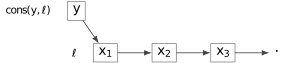
The key consequence is structural sharing. If a list is represented as a chain of pairs, then \(\mathsf{cons}(x,\ell)\) creates one new pair pointing at the old chain \(\ell\); the old list and the new list share everything but that pair, and neither can tell (Figure 3). A structure that needs to “copy” an unbounded old part can instead point to it.
A steque (stack-ended queue) is a sequence supporting push (add at the front), pop (remove the front element), and inject (add at the rear); a catenable steque also supports concatenating two steques [6, pp. 578–579]. A data structure is real-time when every operation takes worst-case constant time—a constant number of primitive steps regardless of the sequence’s length [6, p. 579]. (The reader should keep this data-structure sense of “real-time” apart from the machine sense used in the earlier transfer paper, where a real-time Turing machine is one that performs a bounded number of steps per input letter.) Section 11 quotes the theorem of Kaplan and Tarjan that supplies a purely functional real-time catenable steque.
Algorithms that maintain all palindromes of a growing word use a palindromic tree (the eertree of Rubinchik and Shur [8, §2.2]): one node per distinct palindrome, a suffix link from each node to its longest proper palindromic suffix, and, added whenever it is first discovered, an edge labelled \(c\) from the node of \(P\) to the node of \(cPc\). Discovering that edge means walking suffix links from the current node until a node is found whose occurrence is preceded by \(c\); the walk can be long, but its cost is amortized and the edge is then stored at the old node, so it is never needed again.
A scaffold can do neither thing. It cannot walk an unbounded chain within one step (it sees distance \(k\)), and it cannot add an edge to an old node. The present paper shows what must be stored instead: not a pointer from a palindrome type to a type, but a pointer carried by each occurrence to the particular historical record that the next step will need. Section 7 records, with small counterexamples, why each cheaper idea fails.
This paper builds directly on LMR’s framework. Their scaffolding automata turn the history generated by a finite transition table into an explicit persistent graph, and their correspondence turns acceptance of that graph process into a PEG language. Our question is therefore not only whether \(\mathsf{EPAL}_2\) has some PEG, but which internal recognition dynamic makes palindrome comparison visible to that correspondence.
Finitely Presented Recognition Dynamics, abbreviated FPRD, is the research viewpoint used in this work: a finite grammar or machine description is treated as a presentation that generates an internal recognition dynamic, and the accepted language is treated as one observation of that dynamic. FPRD Lab is the AI-assisted research project in which the present arguments were developed; nothing in this paper requires trust in that project, its tools, or its records, and Section 14 states plainly what was checked by whom. The viewpoint has one concrete role in the proofs: we keep the word-level recurrence (what is true of the input), the record-level representation (what a persistent program stores), and the scaffold-level encoding (what the machine physically appends) as three separate layers, and we prove each implication between them rather than identifying them.
For the prefix \(S\) already read, we factor \(S=CP\) where \(P\) is its longest even-palindromic suffix and retain \(\ell=C^R\). This level contains ordinary words and exact identities.
Palindrome occurrences, typed suffix-link receipts, and receipt ropes expose exactly the historical objects needed by the next transition. Sharing occurs here; a stored receipt is a pointer to a particular record, not merely the name of a palindrome string.
A single physical node tuple-packs all logical records born at one input time. A logical pointer is decoded as a physical historical node plus a finite slot tag.
The distinction between type and occurrence is especially important. The word \(0110\), for example, is one palindrome type. During an online run it may occur at many positions and under different surrounding contexts. A conventional mutable index attaches transitions to the shared type. An immutable scaffold cannot retroactively add a pointer to an old record, so it transports receipts associated with the occurrence that made a transition available. One consequence should be said at once, because it resolves an apparent tension later: the content stored in a record (its suffix link, its bridge letter, its ropes) is a function of the palindrome type alone—the receipt traces of Section 8 are defined from words—so any record of the right type would do semantically; what depends on the occurrence is only which physical record is reachable within the machine’s fixed distance.
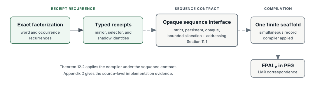
Definitions are given at the first point where they carry proof weight, and Appendix A collects the notation. In diagrams a solid arrow is a logical pointer or implication; a dashed arrow is a decoded or represented relationship rather than an additional heap edge.
Before introducing the record machinery, we follow one word. For every input prefix \(S\), let \(P=P(S)\) be its longest even-palindromic suffix (it exists, since \(\epsilon\) is one), write \(S=CP\), and let \(\ell=C^R\). The pair \((P,\ell)\) determines acceptance: \(\ell=\epsilon\) exactly when the entire prefix is an even palindrome. It also contains enough word-level information to determine the next pair.
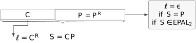
Table 1 gives the complete trace for \(00011001\). The empty word is displayed as \(\epsilon\). “External” means that the new letter matches the first letter of the stored context, so it wraps the entire current palindrome. “Internal” means that the full \(P\) cannot be wrapped, but a proper even-palindromic suffix of \(P\) can. “Reset” means that no even suffix at all—not even the empty one—can be wrapped, so the new longest even suffix is empty. Recall that the empty suffix of a nonempty word counts as preceded by the word’s last letter; that is why row 3 is an internal update and not a reset.
| \(i\) | old \(S\) | \(a\) | old \(P\) | old \(\ell\) | case | new \(P\) | new \(\ell\) |
|---|---|---|---|---|---|---|---|
| 1 | \(\epsilon\) | 0 | \(\epsilon\) | \(\epsilon\) | reset | \(\epsilon\) | 0 |
| 2 | 0 | 0 | \(\epsilon\) | 0 | external | 00 | \(\epsilon\) |
| 3 | 00 | 0 | 00 | \(\epsilon\) | internal | 00 | 0 |
| 4 | 000 | 1 | 00 | 0 | reset | \(\epsilon\) | 1000 |
| 5 | 0001 | 1 | \(\epsilon\) | 1000 | external | 11 | 000 |
| 6 | 00011 | 0 | 11 | 000 | external | 0110 | 00 |
| 7 | 000110 | 0 | 0110 | 00 | external | 001100 | 0 |
| 8 | 0001100 | 1 | 001100 | 0 | internal | 1001 | 1000 |
Two rows are worth pausing over. After the second letter the word is \(00\), so \(P=00\) and the context is empty: the recognizer would accept at that point. The next \(0\) cannot externally wrap \(00\), because there is no letter to its left. Nevertheless the empty proper suffix can be internally wrapped, giving the new longest even suffix \(00\) at the last two positions and context \(0\). At the final row, the current \(P=001100\) is preceded by \(0\), not by the arriving \(1\). The proper suffix \(00\) is preceded inside \(P\) by \(1\), so it is wrapped to \(1001\); the remainder of the old palindrome is transferred into the context. That apparent nonlocal jump is the update that the receipt machinery must make bounded-local.
The case sequence \[\text{reset, external, internal, reset, external, external, external, internal}\] will reappear when we interpret the general recurrence. This word will be followed through every layer of the paper: its row 8 becomes the rope update of Example 8.10 and the scaffold batch of Example 12.1. What generalizes from it is the three-way case split and the use of the empty suffix; what is incidental is the particular word.
Guiding question. What is the smallest exact word state from which one new letter determines the next longest even-palindromic suffix?
Maintaining a longest suffix is reminiscent of a failure-link automaton (a string-matching automaton whose “failure” transitions fall back to the longest matching proper suffix): when the current candidate cannot be extended, one tries a proper suffix. The difference here is that we cannot follow an unbounded chain during one input step. We therefore separate the combinatorial recurrence from the later question of how its selected transition is exposed by one bounded pointer. This section proves the recurrence with ordinary words only.
Let \(S\) be the input prefix read so far. Let \(P(S)\) be its longest even-palindromic suffix and write \[S=CP,\qquad \ell=C^R.\] The word \(\ell\) is the left-context stack of the current occurrence; its first letter lies immediately to the left of \(P\).
Definition 5.1 (selected suffix and displaced chunk). For an even palindrome \(P\) and a letter \(a\), let \(D_a(P)\) be the longest proper even-palindromic suffix \(Q\) of \(P\) for which \[P=ZaQ\] for some word \(Z\) (that is, the longest proper even-palindromic suffix preceded by \(a\) inside \(P\)), and put \(\omega_a(P)=Z^R\). Both are undefined when no such factorization exists.
The pair \((D_a(P),\omega_a(P))\) should be read as a factored transition. Its first coordinate is the longest proper suffix of \(P\) that the arriving \(a\) can wrap. Its second coordinate is exactly the material displaced from the palindrome into the reversed context when that transition is taken. It is important that \(D_a(P)\) is selected by an occurrence of \(a\) immediately before the suffix, not merely by equality of palindrome types.
Definition 5.2 (suffix link, bridge, bridge block). For a nonempty even palindrome \(P\), let \(\lambda(P)\) be its longest proper even-palindromic suffix (possibly \(\epsilon\)), called its suffix link. Write \(P=RbL\) with \(L=\lambda(P)\); the letter \(b\) is the bridge of \(P\) and \(B_P=R^R\) is its bridge block. Because \(P\) and \(L\) are palindromes, \(P=P^R=L^Rb^{}R^R=LbR^R\), so \(L\) is also a prefix of \(P\) and \[P=RbL=LbB_P .\] At the word level we set \(\lambda(\epsilon)=\epsilon\) by convention. At the record level, the typed receipt for this empty word is a distinguished empty record \(\bot\), which has no suffix-link field or bridge. Thus an occurrence of \(\lambda(\epsilon)\) in a word equation means \(\epsilon\), while the same value stored in a receipt slot is represented by \(\bot\).
Example 5.3. For \(P=001100\): \(\lambda(P)=00\), the bridge is \(b=1\) (the letter before the suffix occurrence of \(00\)), \(R=001\), and \(B_P=100\); indeed \(P=001\cdot1\cdot00=00\cdot1\cdot100\). For \(P=0110\): \(\lambda(P)=\epsilon\), \(b=0\) (the last letter), \(R=011\), \(B_P=110\). For \(P=00\): \(\lambda(P)=\epsilon\), \(b=0\), \(B_P=0\).
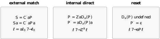
Theorem 5.4 (Occurrence-context factorization). After reading \(a\), the new longest even suffix \(P'\) and reversed context \(\ell'\) are exactly \[(P',\ell')= \begin{cases} (aPa,\ell_0), &\ell=a\ell_0,\\[1mm] (aD_a(P)a,\omega_a(P)\ell), &\ell\notin a\Sigma^*,\ D_a(P)\text{ defined},\\[1mm] (\epsilon,aP\ell), &\ell\notin a\Sigma^*,\ D_a(P)\text{ undefined}. \end{cases}\] Moreover, \[S\in\mathsf{EPAL}_2\quad\Longleftrightarrow\quad \ell=\epsilon.\]
Proof. Strategy. Every new even-palindromic suffix must end with the new letter and therefore begin with it; peel the two copies of \(a\) off and what remains is an old even-palindromic suffix preceded by \(a\). Then maximize.
Every nonempty even-palindromic suffix of \(Sa\) has the form \(aQa\), where \(Q\) is an even-palindromic suffix of \(S\) immediately preceded by \(a\).
If the current longest suffix \(P\) is externally preceded by \(a\), then \(Q=P\) is maximal. Removing that external letter removes the first symbol of \(\ell\). Otherwise every eligible \(Q\) is a proper suffix of \(P\), so maximality selects \(D_a(P)\). Writing \(P=ZaD_a(P)\) shows that the new context is \(CZ\) and hence has reversal \(Z^RC^R=\omega_a(P)\ell\). If no eligible proper suffix exists, the longest even suffix is empty and the reversed full prefix is \(aP\ell\).
Finally \(\ell\) is empty exactly when \(C\) is empty, which is exactly when the whole prefix equals its longest even-palindromic suffix. ◻
In Table 1, rows 2, 5, 6, and 7 are external matches; rows 3 and 8 are internal-direct updates; rows 1 and 4 are resets. The final equivalence in the theorem explains why row 2 is accepting and the final row is not. The theorem also shows why keeping only the length of \(P\) would be insufficient: the internal case must identify a particular suffix and the chunk that precedes it.
Example 5.5 (the two internal rows). At row 3 the old palindrome is \(P=00\) and the context is empty. For the arriving \(0\), the only eligible proper even suffix is \(D_0(P)=\epsilon\). Writing \(P=Z0D_0(P)\) gives \(Z=0\) and \(\omega_0(P)=0\). Hence \(P'=0\epsilon 0=00\) and \(\ell'=0\epsilon=0\). The palindrome type has not changed, but its occurrence has: it now occupies the last two positions of \(000\) rather than all of the preceding prefix. This is a small example of why occurrence context cannot be discarded.
At row 8 the old state is \(S=0001100=0\cdot001100\), \(P=001100\), \(\ell=0\). The arriving letter is \(1\), so the external case fails. The factorization \(P=001\cdot1\cdot00\) shows \(D_1(P)=00\) and \(\omega_1(P)=100\). The recurrence gives \(P'=1\cdot00\cdot1=1001\) and \(\ell'=100\cdot0=1000\). The extra \(1\) in \(Z=001\) is easy to omit when the factorization is read by eye; reversal then makes that omission visible at the front of the new context.
Lemma 5.6 (chunk recursion). Let \(P\) be a nonempty even palindrome with suffix link \(L=\lambda(P)\), bridge \(b\), and bridge block \(B_P\). Then \[D_b(P)=L,\qquad \omega_b(P)=B_P,\] and for every letter \(a\ne b\), \[D_a(P)=D_a(L),\qquad \omega_a(P)=\omega_a(L)\,b\,B_P,\] with the same definedness on both sides (for \(L=\epsilon\) the right-hand sides are undefined).
Proof. Every proper even-palindromic suffix of \(P\) is a suffix of \(L\), since \(L\) is the longest one. The suffix \(L\) itself is preceded by \(b\), so \(D_b(P)=L\) and the displaced chunk is \(R^R=B_P\). For \(a\ne b\), the suffix \(L\) is not eligible, so every eligible suffix is a proper suffix of \(L\) preceded by \(a\) inside \(L\), which is the definition of \(D_a(L)\); writing \(L=Z'aD_a(L)\) gives \(P=RbZ'aD_a(L)\), so \(\omega_a(P)=(RbZ')^R=Z'^R\,b\,R^R=\omega_a(L)\,b\,B_P\). ◻
Example 5.7. For \(P=001100\) (\(L=00\), \(b=1\), \(B_P=100\)): \(D_1(P)=00\), \(\omega_1(P)=100\); and \(D_0(P)=D_0(00)=\epsilon\), \(\omega_0(P)=\omega_0(00)\cdot1\cdot100=0\cdot1\cdot100=01100\). Directly, \(P=00110\cdot0\cdot\epsilon\) and \((00110)^R=01100\).
This recursion is the first sign of persistent self-similarity. For the one letter \(b\) immediately before the suffix link, the desired transition is available at the current record. Every other alphabet coordinate is inherited from the suffix-link record and receives the same intervening block. Because the alphabet is fixed, the entire transition table has fixed width. The remaining difficulty is not the number of coordinates; it is transporting the correct historical record and the potentially long intervening word without walking through either one.
Theorem 5.4 reduces online recognition to catenating type-indexed chunks. It does not yet say how a fresh occurrence obtains its suffix-link record without a search. The needed object is a typed receipt.
A palindrome type is a word such as \(001100\). A palindrome occurrence is that word at a specified interval of the input history. The distinction is inexpensive in the mutable palindromic tree of Section 2.8: a dictionary may map a type and a letter to another type whenever the transition is discovered. An append-only scaffold has no such global update. The record available at the current top must already carry a bounded route to the historical occurrence that will certify its next suffix link.
The word “typed” in typed receipt does not mean a programming-language type annotation. It means that the receipt identifies a record of exactly the palindrome type required by the proof. A raw time coordinate says where some relevant substring ended; a typed receipt says which immutable record at that history node represents the required suffix-link occurrence.
Theorem 6.1 (Typed mirror receipt). Suppose an update selects a longest suffix occurrence \(Q\) of the old input that is immediately preceded by \(a\), and creates \(Y=aQa\). Then \[\lambda(Y)= \begin{cases} aD_a(Q)a,&D_a(Q)\text{ defined},\\ \epsilon,&D_a(Q)\text{ undefined}. \end{cases}\] The palindrome \(\lambda(Y)\) has a complete occurrence in the old input and a pre-existing birth record. One old typed pointer can therefore install the suffix-link field of \(Y\).
Proof. Every proper nonempty even-palindromic suffix of \(Y=aQa\) is \(aRa\), where \(R\) is a proper even-palindromic suffix of \(Q\) immediately preceded in \(Q\) by \(a\). Maximizing \(R\) gives the displayed formula. Since \(Y\) is a palindrome, \(\lambda(Y)\) is also a proper prefix of \(Y\); that prefix ends before the newly appended final \(a\), so the complete occurrence lies in the old input.
At the first occurrence of any nonempty even palindrome \(H\), it is the longest even-palindromic suffix of the prefix ending there. Otherwise a longer even-palindromic suffix would contain \(H\) as a proper prefix as well as a suffix, giving an earlier occurrence of \(H\). The online construction creates a record for the longest even-palindromic suffix at every step, so it has already made a birth record for \(\lambda(Y)\). The empty case uses the distinguished empty record. ◻
Working picture. Reflect the proper suffix of the new palindrome across its center. Its mirror copy finishes before the newly appended last letter, so it is wholly old. The online construction has already created a record when that palindrome first appeared. The receipt transports a pointer to that record rather than asking the next transition to rediscover it.
What this does and does not say. The theorem says that the required record exists in the old history. It does not yet say which old field holds a pointer to it; that is Theorem 8.9(iv): in the external case it is the receipt stored in the first cell of the live context rope, and in the internal case it is the header of the old rope entry selected by the letter. Nor does the theorem say that the pointer reaches the birth record; any record of the right type serves (Section 3).
The word “typed” is essential. A raw endpoint does not identify the needed record at bounded depth. Proposition 6.2 makes this precise for the following endpoint-only discipline: store, instead of a typed pointer, the time at which the mirror copy of the required palindrome ends, and recover the record by starting from the longest even-palindromic suffix of the prefix ending there and following suffix links downward.
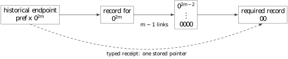
Proposition 6.2 (Endpoint-only escape). For \(m\ge2\), let \(S_m=0^{2m}1100\). Its longest even-palindromic suffix is \(001100\) and the suffix link is \(00\). The mirror occurrence of \(00\) ends at the historical prefix \(0^{2m}\), whose longest suffix-link chain is \[0^{2m},0^{2m-2},\ldots,00,\epsilon.\] Recovering \(00\) from that untyped endpoint takes exactly \(m-1\) suffix-link steps.
Proof. The suffix \(001100\) is an even palindrome, and no longer suffix of \(S_m\) can be a palindrome because any such suffix begins inside the initial zero block but contains its unmatched \(11\) asymmetrically. Its longest proper even suffix is \(00\). The prefix copy of that \(00\) selected by the mirror argument ends at time \(2m\). At that time the input is \(0^{2m}\), whose longest even suffix is the whole prefix and whose proper even suffixes decrease by two zeros at each link. Starting at \(0^{2m}\) reaches \(00\) after \(m-1\) links. ◻
What this does and does not say. This is a representation-specific escape theorem, not a language or scaffold lower bound. It says that the positive construction must transport the typed record pointer itself. What generalizes: any discipline that recovers a record by descending a suffix-link chain from an endpoint is unbounded. What is incidental: the particular family \(0^{2m}1100\).
The receipt construction was not guessed in its final form. Several natural representations preserve enough extensional information to describe the next palindrome but do not expose the needed immutable pointer within a bounded number of old-field traversals. Recording these failures serves two purposes. It explains why the positive representation carries apparently redundant occurrence data, and it keeps the propositions in their proper scope. None of them is a lower bound for PEGs, scaffolding automata, or palindrome recognition in general.
If one record is created at the first birth of each palindrome type, it is tempting to copy a fixed-alphabet transition table from the suffix-link record, as the mutable palindromic tree would do: an entry for letter \(a\) pointing to the record of the target type \(aD_a(P)a\). The target of a later transition, however, need not exist when the source type is born.
Proposition 7.1 (Future transition after type birth). For \(r\geq1\), put \(A_r=0^{2r}\), \[P_r=A_r11A_r, \qquad T_r=1A_r1.\] Then \(D_1(P_r)=A_r\), so the transition selected by \(1\) has target \(T_r=1D_1(P_r)1\). The type \(P_r\) is born by the end of the prefix \(P_r\), but \(T_r\) is not a factor of that prefix. It becomes available only in a later history such as \(P_r1P_r\). Thus the immutable first-birth record of \(P_r\) cannot already point to every future transition out of \(P_r\).
Proof. The word \(A_r\) is the longest proper even-palindromic suffix of \(P_r\) that is immediately preceded by \(1\), giving \(D_1(P_r)=A_r\). Any occurrence of \(T_r=1A_r1\) contains two \(1\) symbols separated by \(2r\) zeros. In \(P_r\) the only adjacent \(1\) symbols lie at its center, so no such factor occurs. In \(P_r1P_r\), the separator \(1\) together with the initial block \(A_r1\) of the second copy gives an occurrence of \(T_r\). This event is strictly later than the birth record of \(P_r\). ◻
The forced design decision is modest but decisive: transitions must be transported by occurrence-indexed receipts, or by some representation of equal strength. A canonical type node remains useful for explaining suffix relations, but it is not by itself a closed immutable update interface. The reader may ask why the per-letter entries that the final construction does store (Section 12) escape this proposition. They do because they point to the record of the selected suffix \(D_a(P)\), which exists when \(P\) is born (it is a suffix of \(P\)), and not to the record of the target \(aD_a(P)a\), which may not.
A persistent rope can share the letters of a context perfectly. Receipts, however, depend on the palindrome around which those letters are interpreted.
Proposition 7.2 (Anchor dependence). For the fixed one-letter block \(w=0\) and anchors \(A_r=0^{2r}\), \[\lambda(0A_r0)=A_r.\] Consequently the same raw rope cell \(0\) requires infinitely many distinct typed receipt targets as its anchor varies.
Proof. The word \(0A_r0=0^{2r+2}\) is an even palindrome. Its longest proper even palindromic suffix is \(0^{2r}=A_r\). These target types are distinct as \(r\) varies. Hence a receipt attached only to the raw letter block cannot be correct for all anchors. ◻
This proposition does not forbid structural sharing of the underlying word. It says that the positive object must be an anchored receipt path, and that later reuse must justify why the receipt shadow survives a legal change of physical anchor. Lemma 8.3 supplies exactly that justification.
One might defer the missing transition and repeatedly follow the suffix link, testing the bridge letter at each record. The following family makes the number of failed tests arbitrary.
Proposition 7.3 (Bridge-chasing escape). For \(r\geq1\) and \(d\geq0\), let \[P_{r,d}=A_r(11A_r)^d, \qquad A_r=0^{2r}.\] These are even palindromes. For \(d>0\), \[\lambda(P_{r,d})=P_{r,d-1} \quad\text{and}\quad b_{P_{r,d}}=1,\] whereas the bridge of \(A_r\) is \(0\). The search for the \(0\)-transition from \(P_{r,d}\) therefore makes exactly \(d\) failed bridge tests before reaching the variable target \(A_r\).
Proof. The word \(P_{r,d}=A_r11A_r11\cdots11A_r\) is unchanged by reversal, so it is an even palindrome. The suffix beginning after the first block \(A_r11\) is \(P_{r,d-1}\) and is palindromic. No longer proper suffix is palindromic: a suffix beginning inside the first \(A_r\) has fewer initial zeros than terminal zeros and meets a \(1\) while its reversal is still inside the terminal zero block; a suffix beginning in the following \(11\) starts with \(1\) and ends with \(0\). Hence \(P_{r,d-1}\) is the longest proper even-palindromic suffix. The letter immediately before it is the second \(1\) of the removed \(11\) block.
Thus each of the first \(d\) records rejects the requested bridge letter \(0\) and delegates to its suffix link. At \(P_{r,0}=A_r\), the bridge letter before its longest proper even suffix is \(0\) (for \(r=1\), \(\lambda(00)=\epsilon\) is preceded by the last letter \(0\)), so the recursion stops. There are exactly \(d\) failures, and \(d\) is unbounded. ◻
The proposition refutes bounded bridge chasing for this representation. It does not refute recursively stored direct transitions: the final construction materializes the same recursion persistently, so the transition selected in a later step is already at bounded depth.
| Attempt | What it preserves | Escape family | Information retained finally |
|---|---|---|---|
| Historical endpoint | where the mirror copy ends | \(0^{2m}1100\): target \(00\) lies \(m-1\) links below the historical maximum | direct typed pointer to the required record |
| Immutable type-birth table | canonical suffix-link type | \(P_r=0^{2r}11 0^{2r}\): a needed target is born later | occurrence-indexed transition receipt |
| Anchor-free word rope | persistent raw context letters | the block \(0\) over anchors \(0^{2r}\) needs different receipts | headered anchored receipt path |
| Bounded bridge chase | correct recursive selector equation | \(P_{r,d}\) forces exactly \(d\) failures | persistently materialized direct/reset rope |
These eliminations narrow the task to a positive one: define an anchored path whose cells carry typed receipts, and prove that the parts shared after an online update retain the same receipt trace even when their concrete palindrome anchors change. That is the purpose of receipt ropes.
Guiding question. How can a persistent sequence share an arbitrarily long old tail when the palindrome at the tail’s central anchor has changed?
Consider the current state \((P,\ell)\) with \(\ell=c_1c_2\cdots c_k\). If the next input letters happen to be \(c_1,c_2,\ldots\) in that order, the external case of Theorem 5.4 fires each time: the palindrome becomes \(c_1Pc_1\), then \(c_2c_1Pc_1c_2\), and so on, while the context loses one letter each time. Each of those future palindromes will need its suffix link at the moment it becomes current (Theorem 6.1), and each is determined by \(P\) and a prefix of \(\ell\). A receipt rope stores the context as a sequence of cells, one per context letter, where cell \(i\) carries both the letter \(c_i\) and the typed receipt for the palindrome obtained after \(i\) external matches. Popping a cell (an external match) then exposes, in the next cell, exactly the receipt the new current palindrome needs. The rope is not merely a word with annotations: it is a walk through palindrome occurrences, anchored at \(P\).
The record at the front is a header: the receipt of the anchor itself. If a pop makes the first wrapped palindrome current, its suffix-link receipt is promoted to the new header. This promotion is what an ordinary list of letters lacks.
Definition 8.1 (anchored path, receipt trace, headered rope). For an even palindrome \(A\) and a word \(w=c_1\cdots c_k\), define the anchored path \(\Pi(A,w)\) by \[A_0=A,\qquad A_i=c_iA_{i-1}c_i ,\] and write \(\operatorname{wrap}_w(A)=A_k\) for its final palindrome. Cell \(i\) of the path stores \((c_i,\lambda(A_i))\). Its receipt trace is \[\Lambda(A,w)=(\lambda(A_1),\ldots,\lambda(A_k)),\] and its headered form is \[\widehat\Pi(A,w)= \bigl(\lambda(A);(c_1,\lambda(A_1)),\ldots,(c_k,\lambda(A_k))\bigr),\] whose first component is the header and whose sequence of cells is the body. Palindrome words in a receipt position denote typed pointers to the particular occurrence records supplied by the construction, not mere type tags. In particular, the displayed header \(\lambda(\epsilon)=\epsilon\) of a rope anchored at \(\epsilon\) is physically represented by \(\bot\).
The header is the receipt required if the anchor becomes current; taking a tail promotes the first cell’s receipt to the new header. Anchored paths obey the literal catenation law \[\Pi(A,uv)=\Pi(A,u)\cdot\Pi(\operatorname{wrap}_u(A),v).\] The catenation law carries an important guard: the second path is anchored at the result of wrapping \(A\) by \(u\). Two identical raw words do not therefore represent interchangeable receipt ropes at arbitrary anchors. Proposition 7.2 is the one-letter instance of this fact.
Example 8.2. The live context at row 7 of Table 1 is \(\widehat\Pi(001100,0)=(00;\,(0,00))\): the header is \(\lambda(001100)=00\), and the one cell records that after an external match by \(0\) the palindrome \(00011000\) would have suffix link \(00\).
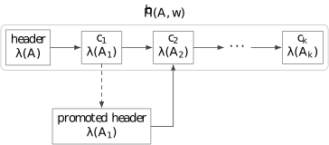
The physical palindrome states in a retained context tail can change after a prepend or reset. The next lemma shows that the typed receipt trace does not. Its two anchors \(H\) and \(P\) are different words; the claim is that wrapping them through the same context produces the same sequence of suffix links.
Lemma 8.3 (Bridge-shadow identity). Suppose \(H=RbP\), \(\lambda(H)=P\), and \(P\) is the longest even-palindromic suffix of \(w^RP\). If \(w=\epsilon\), or if the first letter of \(w\) differs from \(b\), then \[\Lambda(H,w)=\Lambda(P,w).\]
(The statement allows \(P=\epsilon\): then \(H=Rb\) is any nonempty even palindrome with \(\lambda(H)=\epsilon\), and the hypothesis on \(w^RP=w^R\) says \(w^R\) has no nonempty even-palindromic suffix.)
Example 8.4. \(H=0000\), \(P=\lambda(H)=00\), \(b=0\), \(w=1\): the hypotheses hold (\(1\ne0\); \(w^RP=100\) has longest even-palindromic suffix \(00\)), and indeed \(\lambda(1\,0000\,1)=\epsilon=\lambda(1\,00\,1)\).
Working picture. The anchors \(H\) and \(P=\lambda(H)\) begin with the same suffix-link choice as soon as the first context letter is not the bridge \(b\). If their receipt traces first diverged later, the unequal bridge exposed at that first divergence could be reflected through the context already consumed. The reflection would form an even-palindromic suffix strictly longer than \(P\) in \(w^RP\), contradicting the hypothesis that \(P\) is longest. The proof below adds indices and a strict length bound to this picture.
Proof. Strategy. Compare the two wrapped words cell by cell. Both end in the same suffix; as long as the receipt is strictly shorter than that common suffix, the next bridge letter is read inside it and the two sides agree. The only way the receipt could grow to the full common length is excluded by the maximality hypothesis.
For a letter \(c\) and even palindrome \(X\), put \(G_c(X)=\lambda(cXc)\). Every proper even-palindromic suffix of \(X\) is a suffix of \(\lambda(X)\). Hence \[G_c(X)= \begin{cases} c\lambda(X)c,&c\text{ is the bridge before }\lambda(X),\\ G_c(\lambda(X)),&\text{otherwise}. \end{cases} \tag{1}\]
Write \(w=c_1\cdots c_k\), put \(u_i=c_1\cdots c_i\), and define \[X_i=u_i^RHu_i,\qquad Y_i=u_i^RPu_i,\qquad N_i=|P|+i.\] Both \(X_i\) and \(Y_i\) end in the same word \(T_i=Pu_i\), of length \(N_i\). We prove for every \(i\geq1\) that \[\lambda(X_i)=\lambda(Y_i)=K_i \quad\hbox{and}\quad |K_i|<N_i. \tag{2}\]
For \(i=1\), the hypothesis \(c_1\ne b\) and (1) give \(G_{c_1}(H)=G_{c_1}(P)\). This common palindrome is a proper suffix of \(c_1Pc_1\), so its length is at most \(|P|<N_1\).
Assume (2) at \(i<k\). Since \(K_i\) is shorter than the common suffix \(T_i\), the letter immediately before its terminal occurrence lies inside \(T_i\). It is therefore the same bridge letter in \(X_i\) and \(Y_i\). Equation (1), with \(c=c_{i+1}\), now gives the same next receipt on both sides: it is either \(cK_ic\) when \(c\) is that common bridge, or \(G_c(K_i)\) otherwise.
It remains to retain the strict length bound. In the second case \(|G_c(K_i)|\leq |K_i|<N_i<N_{i+1}\). In the first case the only way \(|cK_ic|\) could reach \(N_{i+1}\) is, by parity, that \(N_i\) is odd and \(|K_i|=N_i-1\). Then the common suffix has the form \(T_i=cK_i\). Because \(K_i\) is a palindrome, \[(u_ic)^RP=c\,u_i^RP=cT_i^R=cK_ic\] is an even-palindromic suffix of \(w^RP\) strictly longer than \(P\): the word \(u_ic\) is a prefix of \(w\). This contradicts the maximality hypothesis. Thus (2) follows by induction, and its receipt equalities are precisely \(\Lambda(H,w)=\Lambda(P,w)\). ◻
The length inequality in (2) is not bookkeeping decoration. It ensures that the bridge inspected at the next step lies inside the suffix shared by both physical anchors. The parity subcase is the only point at which equality could occur; resolving it by constructing the forbidden longer suffix is what makes the shadow statement global rather than merely a one-cell observation.
For nonempty \(Y\) with suffix link \(L\), bridge \(b\), and bridge block \(B\), write \[Y=RbL=LbB.\] When \(D_c(Y)\) is defined, define the direct headered rope \[\Omega_c(Y)= \widehat\Pi\bigl(cD_c(Y)c,\omega_c(Y)\bigr).\] When it is undefined, define the reset rope \[Z_c(Y)=\widehat\Pi(\epsilon,cY).\] The direct rope is the context rope that the internal case of Theorem 5.4 will need: it is anchored at the palindrome \(cD_c(Y)c\) that the letter \(c\) creates, and its cells carry the receipts for the displaced chunk \(\omega_c(Y)\) that becomes the front of the new context. The reset rope is the analogue when nothing can be wrapped: anchored at \(\epsilon\), its cells carry the receipts for the whole failed candidate \(cY\).
The last cell of such a rope has a receipt that can be named explicitly. This fact is used three times below (in Theorems 8.7 and 8.9), so we state it once.
Lemma 8.5 (Mirror-prefix lemma). Let \(Y\) be a nonempty even palindrome and \(c\) a letter.
If \(D_c(Y)\) is defined, the final palindrome of \(\Pi(cD_c(Y)c,\omega_c(Y))\) is \(F=Yc\,\omega_c(Y)\), and \(\lambda(F)=Y\).
If \(D_c(Y)\) is undefined, the final palindrome of \(\Pi(\epsilon,cY)\) is \(F=YccY\), and \(\lambda(F)=Y\).
In both cases the last receipt of the rope is the anchor’s source \(Y\) itself.
Proof. (1) Write \(Y=ZcD\) with \(D=D_c(Y)\) and \(\omega=\omega_c(Y)=Z^R\). Wrapping \(cDc\) through \(\omega\) gives \(F=\omega^R\,cDc\,\omega=ZcDcZ^R=YcZ^R\). Since \(F\) is a palindrome with prefix \(Y\), the word \(Y=Y^R\) is also a suffix of \(F\), and it is a proper even-palindromic suffix. Suppose a longer proper even-palindromic suffix \(V=yY\) existed, with \(y\) a nonempty suffix of \(Zc\), \(|y|\) even. Palindromicity of \(V\) gives \(yY=Yy^R\), so \(Y\) has period \(|y|\): its suffix \(Y''\) of length \(|Y|-|y|\) equals its prefix of that length, and since \(Y\) is a palindrome that prefix is the reversal of \(Y''\); hence \(Y''\) is an even palindrome. The same equality identifies \(y\) with the prefix of \(Y\) of length \(|y|\), so the terminal occurrence of \(Y''\) in \(Y\) is preceded by the last letter of \(y\), which is \(c\) because \(y\) is a suffix of \(Zc\). By maximality of \(D=D_c(Y)\), \(|Y''|\le|D|\), i.e. \(|y|\ge|Y|-|D|=|Z|+1\); so \(y=Zc\) and \(V=F\) is not proper, a contradiction.
(2) Wrapping \(\epsilon\) through \(cY\) gives \(F=(cY)^R\epsilon\,(cY)=YccY\), a palindrome with prefix \(Y\), so \(Y\) is a proper even-palindromic suffix. If a longer proper one \(V=yY\) existed, with \(y\) a nonempty suffix of \(Ycc\) of even length, the same periodicity argument shows that the suffix \(Y''\) of \(Y\) of length \(|Y|-|y|\) is an even palindrome. When \(|y|\le|Y|\), the equality \(yY=Yy^R\) identifies \(y\) with the corresponding prefix of \(Y\); because \(y\) ends in \(c\), the terminal occurrence of \(Y''\) is preceded by \(c\), which would make \(D_c(Y)\) defined. And \(|y|>|Y|\) forces \(|y|=|Y|+2\), i.e. \(V=F\), not proper. ◻
Corollary 8.6. With \(Y=LbB\) as above and \(c\ne b\): if \(D_c(Y)\) is defined, write \(L=ZcD_c(L)\); then \(\lambda(ZcL)=L\). If \(D_c(Y)\) is undefined, then \(\lambda(LccL)=L\).
Proof. By Lemma 5.6, \(D_c(Y)\) is defined iff \(D_c(L)\) is (for \(L=\epsilon\) both are undefined). Apply Lemma 8.5 to \(L\) in place of \(Y\): the final palindrome of \(\Pi(cD_c(L)c,\omega_c(L))\) is \(ZcL\), and that of \(\Pi(\epsilon,cL)\) is \(LccL\). (For \(L=\epsilon\) the second case reads \(\lambda(cc)=\epsilon\).) ◻
Theorem 8.7 (Receipt-rope recurrence). Let \(\rho_b\) be the header receipt of \(\Omega_b(Y)\). For \(c\ne b\), \[\Omega_c(Y)= \begin{cases} \text{undefined},&\Omega_c(L)\text{ undefined},\\ \Omega_c(L)\cdot(b,\rho_b)\cdot\operatorname{body}\Omega_b(Y),&\text{otherwise}, \end{cases}\] and, whenever \(Z_c(Y)\) is defined, \[Z_c(Y)=Z_c(L)\cdot(b,\rho_b)\cdot\operatorname{body}\Omega_b(Y).\]
In words, every off-bridge direct rope and every reset rope consists of three pieces already visible at bounded depth: the corresponding rope at the suffix link \(L\), one bridge cell, and the body of the single bridge-matching rope at \(Y\). The bridge-shadow identity is what makes the third piece literally shareable; without it the equation would describe only equal raw words and would not be a persistent pointer construction. Note that the third piece is shared between two ropes whose anchors differ: in \(\Omega_c(Y)\) the cells after the bridge cell are anchored at \(b\,(ZcL)\,b\), in \(\Omega_b(Y)\) at \(bLb\).
Proof. Strategy. The raw words agree by Lemma 5.6; the receipts of the shared tail agree by the bridge-shadow identity applied to all cells but the last, and the last receipts agree by the mirror-prefix lemma.
Raw words. Let \(c\ne b\). By Lemma 5.6, \(D_c(Y)=D_c(L)\) with the same definedness, and \(\omega_c(Y)=\omega_c(L)\,b\,B\). Hence, when defined, \(\Omega_c(Y)\) is anchored at the same palindrome \(cD_c(L)c\) as \(\Omega_c(L)\) and wraps through \(\omega_c(L)\), then \(b\), then \(B\); by the catenation law its first \(|\omega_c(L)|\) cells are literally those of \(\Omega_c(L)\), its next cell has letter \(b\), and its remaining cells are \(\Pi(H',B)\) where \(H'=b\,\operatorname{wrap}_{\omega_c(L)}(cD_c(L)c)\,b=b(ZcL)b\) with \(L=ZcD_c(L)\). In the reset case, \(Z_c(Y)=\widehat\Pi(\epsilon,cLbB)\) similarly begins with the cells of \(Z_c(L)=\widehat\Pi(\epsilon,cL)\), continues with a \(b\) cell, and ends with \(\Pi(H',B)\) where \(H'=b(LccL)b\). On the other side, \(\operatorname{body}\Omega_b(Y)=\Pi(bLb,B)\) since \(D_b(Y)=L\) and \(\omega_b(Y)=B\).
Receipts. Put \(H=ZcL\) (direct case) or \(H=LccL\) (reset case), so that \(H'=bHb\), and write \(B=B'x\) with \(x\) its last letter (\(B\) is nonempty because \(|Y|-|L|-1\ge1\)). We claim \(\Lambda(H,bB)=\Lambda(L,bB)\); the first entry of this identity is the statement that the \(b\) cell of \(\Omega_c(Y)\) (resp. \(Z_c(Y)\)) carries \(\lambda(bLb)=\rho_b\), and the remaining entries identify \(\Pi(H',B)\) with \(\Pi(bLb,B)\) receipt by receipt.
Apply Lemma 8.3 with \(H\), \(P:=L\), and \(w:=bB'\). Its hypotheses hold: \(H=R'cL\) has bridge \(c\ne b\) and \(\lambda(H)=L\) by Corollary 8.6; and \(w^RL=B'^RbL\) is \(Y\) with its first letter removed, whose even-palindromic suffixes are exactly the proper even-palindromic suffixes of \(Y\), the longest being \(L\). The lemma gives agreement of the receipts on all cells except the last. For the last cell, the final palindromes are \(Yc\,\omega_c(Y)\) (resp. \(YccY\)) on the left and \(YbB\) on the right; both have suffix link \(Y\) by Lemma 8.5. Hence \(\Lambda(H,bB)=\Lambda(L,bB)\), which is the displayed identity.
Definedness. \(\Omega_c(Y)\) is defined iff \(\Omega_c(L)\) is, by Lemma 5.6; and \(Z_c(Y)\) is defined (i.e. \(D_c(Y)\) undefined) iff \(Z_c(L)\) is. ◻
Example 8.8 (the recurrence on \(Y=001100\)). Here \(L=00\), \(b=1\), \(B=100\). For \(c=0\): \(\Omega_0(L)=\widehat\Pi(00,0)=(\epsilon;(0,00))\), \(\Omega_1(Y)=\widehat\Pi(1001,100)=(\epsilon;(1,11),(0,0110),(0,001100))\), so \(\rho_1=\epsilon\) and the recurrence predicts \(\Omega_0(Y)=(\epsilon;(0,00),(1,\epsilon),(1,11),(0,0110),(0,001100))\). Direct computation of \(\widehat\Pi(00,01100)\) gives the same five cells. The shared tail is anchored at \(1\,0000\,1\) on the left and at \(1\,00\,1\) on the right; the two anchors differ, and their receipts agree.
Theorem 8.9 (Full abstract receipt closure). Over a fixed alphabet, every nonreset update obtains a fresh occurrence record, its complete direct/reset rope table, and the updated live context from old receipts by a fixed number of head, tail, singleton, inject, and catenation operations. On reset, only the live rope is updated and the occurrence root becomes the fixed empty record.
The adjective “abstract” marks a clean interface boundary. The theorem has already eliminated suffix-link search, mutation, global interning, and random access to the old input. It assumes only a persistent sequence supporting a fixed collection of operations in worst-case bounded structural work. The next part supplies that sequence and explains how its fresh structural records are represented by the scaffold. Which old fields hold the receipts named below is fixed by the record layout of Section 12.
Proof. Strategy. Build the fresh record’s bridge rope from one old rope by one pop and one inject; build its other entries by Theorem 8.7; build the new live context by Theorem 5.4.
Suppose the update creates \(P=aQa\), where \(Q\) is the old longest suffix (external case) or \(Q=D_a(P_{\mathrm{old}})\) (internal case), and let \(L=\lambda(P)\) as given by Theorem 6.1. Select the old rope \(\Omega_a(Q)\) when \(D_a(Q)\) is defined and the old reset rope \(Z_a(Q)\) otherwise; call it the source rope. Its body is nonempty (its word is \(\omega_a(Q)\), resp. \(aQ\), and both are nonempty); write the body \((b,H)\mathcal T\).
The bridge of \(P\) is \(b\). If \(D_a(Q)\) is defined, write \(Q=Z'aD_a(Q)\); then \(P=aZ'\,aD_a(Q)a=(aZ')L\), so the bridge of \(P\) is the last letter of \(Z'\), which is the first letter of \(\omega_a(Q)=Z'^R\), i.e. \(b\). If \(D_a(Q)\) is undefined, \(L=\epsilon\), the bridge of \(P\) is its last letter \(a\), and the first letter of the reset rope’s word \(aQ\) is \(a=b\).
The header of \(\Omega_b(P)\) is \(H\). The header of \(\Omega_b(P)=\widehat\Pi(bLb,\omega_b(P))\) is \(\lambda(bLb)\). The first cell of the source rope is obtained by wrapping its anchor (\(aD_a(Q)a=L\), resp. \(\epsilon=L\)) by \(b\), so its receipt is \(H=\lambda(bLb)\).
The body of \(\Omega_b(P)\) is \(\mathcal T\) followed by \((a,P)\). By (i), \(P=(aZ''b)L\) with \(Z'=Z''b\), so \(\omega_b(P)=Z''^Ra\), while the source rope’s word is \(\omega_a(Q)=Z'^R=bZ''^R\) (in the reset case \(\omega_a(P)=Qa\) and the source word is \(aQ\)). So \(\Omega_b(P)\) wraps \(bLb\) through the same letters as the source rope after its first cell, followed by one final letter \(a\). By the catenation law the cells coincide with \(\mathcal T\), and the final cell has letter \(a\) and receipt \(\lambda(\operatorname{wrap}_{\omega_b(P)}(bLb))=P\) by Lemma 8.5. In symbols, \[b_P=b,\qquad \Omega_b(P)=\bigl(H;\mathcal T(a,P)\bigr). \tag{2}\] Operationally: pop the source body, inject the terminal cell \((a,P)\), and reuse the old header \(H\).
The suffix-link pointer of \(P\). In the external case \(Q=P_{\mathrm{old}}\) and \(L=\lambda(aP_{\mathrm{old}}a)\) is the receipt stored in the first cell of the live rope \(\mathcal K(P_{\mathrm{old}},\ell)\), which the pop of (3) below promotes to the new header. In the internal case \(L=\lambda(aD_a(P_{\mathrm{old}})a)\) is the header of the old entry \(\Omega_a(P_{\mathrm{old}})\), whose anchor is \(aD_a(P_{\mathrm{old}})a=P\). In both cases one old receipt names a record of type \(L\).
Every other entry of the fresh record follows from (2), Theorem 8.7, and the finite alphabet: for \(c\ne b\), the rope \(\Omega_c(P)\) or \(Z_c(P)\) is \(\Omega_c(L)\) (resp. \(Z_c(L)\)) catenated with the singleton \((b,H)\) and with \(\operatorname{body}\Omega_b(P)\)—two catenations on ropes read from the record of \(L\), which is reached by the pointer of (iv). The bridge transition receipt is the suffix-link receipt \(L\); every off-bridge direct transition receipt is copied from the corresponding entry of the record for \(L\).
Let \(\mathcal K(P,\ell)=\widehat\Pi(P,\ell)\) be the live context rope. The three cases of Theorem 5.4 give \[\mathcal K'= \begin{cases} \operatorname{tail}\mathcal K(P,\ell),&\ell=a\ell_0,\\ \Omega_a(P)\cdot\operatorname{body}\mathcal K(P,\ell), &D_a(P)\text{ defined},\\ Z_a(P)\cdot\operatorname{body}\mathcal K(P,\ell), &D_a(P)\text{ undefined}, \end{cases} \tag{3}\] where \(P\) denotes the old palindrome. The first case is the catenation law read backwards. In the second case the new live rope is \(\widehat\Pi(aD_a(P)a,\omega_a(P)\ell)=\Omega_a(P)\cdot\Pi(\operatorname{wrap}_{\omega_a(P)}(aD_a(P)a),\ell)\), and the tail is anchored at \(H:=ZaP\) where \(P=ZaD_a(P)\); in the third case the tail is anchored at \(H:=PaaP\). Lemma 8.3 applies to \(H\), \(P\), and \(w:=\ell\): \(\lambda(H)=P\) by Lemma 8.5 (applied to \(P\) and \(a\)), the bridge of \(H\) is \(a\), either \(\ell=\epsilon\) or its first letter differs from \(a\), and \(w^RP=\ell^RP=CP=S\), of which \(P\) is the longest even-palindromic suffix by definition. So the old body is literally reusable even though its concrete anchor changes. Equations (2)–(3) use a fixed number of rope primitives and old fields. ◻
Example 8.10 (row 8 at the rope layer). Before row 8 the state is \(P=001100\), \(\ell=0\), with live rope \(\mathcal K=(00;(0,00))\). The letter is \(a=1\), the internal case with \(Q=D_1(001100)=00\), and the fresh palindrome is \(P'=1001\). The source rope is \(Z_1(00)=(\bot;(1,\epsilon),(0,\epsilon),(0,00))\) since \(D_1(00)\) is undefined; so \(b=1\), \(H=\epsilon\), \(\mathcal T=((0,\epsilon),(0,00))\), and (2) gives \[\Omega_1(1001)=\bigl(\epsilon;\ (0,\epsilon),(0,00),(1,1001)\bigr),\] which agrees with the direct definition \(\widehat\Pi(11,001)\). The suffix-link pointer of the fresh record is the header of \(\Omega_1(001100)=(\epsilon;(1,11),(0,0110),(0,001100))\), namely \(\epsilon\), the empty record. The new live rope by (3) is \[\mathcal K'=\Omega_1(001100)\cdot\operatorname{body}\mathcal K =\bigl(\epsilon;\ (1,11),(0,0110),(0,001100),(0,00)\bigr),\] which is \(\widehat\Pi(1001,1000)\) computed directly. The last cell \((0,00)\) was created at row 7 around the anchor \(001100\) and is now read around the anchor \(1001\); its receipt is unchanged. The terminal cell \((1,1001)\) of the fresh bridge rope points at the fresh record itself: this is the cycle of Part III. What generalizes: every nonreset update has exactly this shape. What is incidental: the particular lengths.
Guiding question. If every rope operation performs only bounded work, why can we not simply allocate its fresh immutable records in topological order?
From here on a record is a finite tuple with a finite tag, a finite payload (such as a letter), and a fixed number \(q\) of pointer fields, each of which is missing or points to a record. A persistent program holds a fixed number \(s\) of roots (pointers kept in finite control) and, at each step, reads old records by following fields from the roots and creates a finite batch of fresh records. The fresh batch is a finite labelled directed graph: its vertices are the fresh records (slots \(0,\ldots,A-1\) for some bound \(A\)), and each field of each slot is missing, points to an old record, or points to a slot.
In ordinary functional programming a fresh record can only point to records that already exist when its constructor runs, so the fresh batch of one step is acyclic and can be allocated in topological order: first the records with no fresh targets, then those pointing only to them, and so on. Three small batches show what a cycle would mean. A self-loop has one slot \(x\) with field \(f(x)=x\). A forward reference has two slots \(x,y\), created in that order, with \(f(x)=y\). A mutual cycle has \(f(x)=y\) and \(g(y)=x\). All three are perfectly good finite labelled adjacency tables; none can be produced by allocating one constructor at a time, because the first constructor would have to store a pointer to a record that does not exist yet.
The obstruction is already visible in equation (2) of the closure proof. A fresh palindrome occurrence record \(P\) stores the root of its bridge rope \(\Omega_b(P)\). The final fresh cell of that rope stores the typed receipt \(P\). Thus \[P\longrightarrow\Omega_b(P) \longrightarrow\text{terminal receipt }P.\] Both edges are semantic requirements of the same input transition. Neither endpoint can be replaced by an old record, and neither ordering of the two fresh objects makes all pointers backward. Example 8.10 exhibits the cycle concretely: the record for \(1001\) and the cell \((1,1001)\) are both created at row 8 and point at each other.
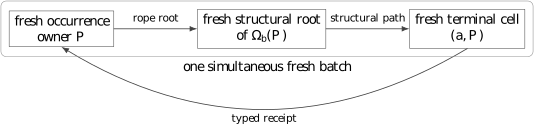
This is not a request for a recursively defined infinite object. After the input letter and bounded old observation are fixed, there are finitely many fresh slots and a finite adjacency table saying which slot each field targets. The graph may contain a cycle, exactly as an ordinary finite directed graph may. Decoding the graph means recovering that adjacency table; it does not mean recursively unfolding the cycle into a tree.
A previously considered source interface allowed a fresh field to name only an old object or an earlier fresh slot. That interface silently excludes Figure 9; proving closure inside it would prove a theorem about the wrong program. The repair is to permit arbitrary references within one uniformly bounded fresh batch and then show that this stronger source step still compiles to the target model. The palindrome batch is larger than the three toy batches but no different in kind.
We now define the source machine precisely and compile it into the scaffold model of Definition 2.6. This section is independent of palindromes: a reader may regard its input as an arbitrary bounded persistent-record update.
Definition 10.1 (Bounded simultaneous record transducer). Fix constants \(s,A,q,r\). A bounded simultaneous record transducer has \(s\) current roots, allocates at most \(A\) active slots per input symbol, gives each record \(q\) pointer fields, and follows at most \(r\) old-record fields from its current roots in one step. Its control states, record tags, and nonpointer payloads are finite.
After its bounded old observation, one transition chooses a finite labelled batch graph. Every new root and field targets one of: \[\varnothing,\qquad \text{an old address of at most $r$ dereferences},\qquad \text{any active slot of the fresh batch}.\] The last case includes self-loops, forward references, and mutual cycles. The whole finite adjacency table is specified simultaneously. No fresh record is inspected while the plan is chosen, and control does not branch on whether two old addresses name the same record.
An old address is a root together with a sequence of at most \(r\) field names; it is dereferenced by starting at the root and following the named fields. “Simultaneous” constrains dependencies rather than prescribing a physical allocation primitive. The plan may depend on finite control and bounded old structure, but it may not branch on a fresh record as though that record had already been evaluated. The adjacency table is output data of the transition. The initial roots may be missing or point into a fixed finite, immutable, pointer-closed initial record graph. The compiled decoder stores that graph and its initial roots as finite table data; those virtual records are present from time zero and are never charged to a fresh batch.
The scaffold appends one node per letter; the transducer creates up to \(A\) records per letter. Tuple packing resolves the tension: the one physical node \(v_t\) appended at time \(t\) represents the entire batch born at time \(t\), and a finite slot number \(i<A\) says which logical record is meant. A logical pointer is decoded as a pair \((v_t,i)\). The physical node’s label records, for each of its ports, the slot number of the record that port’s target stands for; old logical field traversal therefore alternates between a physical port and the finite slot tag read at the node that owns the port. A fresh pointer uses \(\mathsf{SELF}\) to return to \(v_t\) and carries the desired fresh slot in the new label. The physical graph remains a legal scaffold; “record” is an interpretation placed on its ports and label.
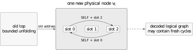
Theorem 10.2 (Simultaneous batch compiler; corrected initialization case). Every transducer of Definition 10.1 whose initial record graph is fixed, finite, immutable, and pointer-closed compiles exactly and letter-synchronously into a finite scaffolding automaton of degree \[d=\max\{1,s+Aq\}\] and observation/update distance at most \(r+1\). The source transition uses only bounded labelled rooted unfoldings and does not branch on pointer identity; acceptance is in finite control.
Reading note. The dynamic tuple-packing argument below is retained. Its former missing-root base case is replaced by the virtual-initial-record argument above.
Proof. Strategy. Fix the encoding (ports for roots and fields, slot tags in labels); show that every old address compiles to a port word of length at most \(r+1\) that the transition can compute from its neighbourhood; show that the decoded fresh batch equals the source batch as a finite labelled graph; then induct on the input.
One physical scaffold node represents the complete logical batch at one input time. Its finite label records the active mask, every tag and payload, and for each of its \(d\) ports the finite target-slot tag of the record that port stands for (when the target is present).
Ports \(0,\ldots,s-1\) represent the next roots. Port \(s+iq+j\) represents field \(j<q\) of slot \(i<A\). Thus a decoded logical pointer is a pair \((v,i)\) of a physical scaffold node and a finite slot number.
Consider an old logical address that starts at root \(u\) and follows fields \(j_1,\ldots,j_m\), with \(m\le r\). The current labelled unfolding reveals the slot reached after every prefix, because each slot tag is stored in the label of the node whose port is being followed, and that node lies within distance \(m\le r\) of the old top. Compile the address to the raw port word \[u,\ s+i_0q+j_1,\ \ldots,\ s+i_{m-1}q+j_m,\] where \(i_h\) is the slot tag at the preceding logical pointer. This word has length at most \(r+1\) and reaches exactly the old target. The extra one in the distance bound is the initial root port; each logical dereference contributes one field port thereafter. LMR’s transition sees the labels of all nodes within distance \(k\) (Definition 2.5), so \(k=r+1\) suffices both to compute the word and to read the tags along it.
Use a missing descriptor for \(\varnothing\) and the compiled word for an old target. For every fresh target use physical \(\mathsf{SELF}\) and record the intended logical slot in the new finite label. This rule makes no distinction between an earlier target, a later target, a self-loop, or one edge of a mutual cycle.
Assume that the old top decodes to the source roots and old heap. Induction on the length of an old logical address proves that its raw word decodes correctly: the base root port reaches the physical node named by that root and supplies its slot; each subsequent field port is selected using the current slot and supplies the next slot. Missing decodes to missing. A fresh descriptor reaches the new physical node by \(\mathsf{SELF}\) and then its target-slot tag selects exactly the requested fresh logical record.
Applying these facts independently to every root and field makes the decoded finite labelled adjacency table identical to the source batch. Notice that the induction is on an old address, never on the unfolding of a fresh cycle. Comparing two finite adjacency tables requires no fixed point. Tags, payloads, control, and acceptance are copied directly.
The virtual-initial-record base case and this one-step commuting square give the full run invariant by induction on input length. All parameter ranges, masks, labels, and plans are finite, so the compiled automaton is finite. ◻
For the three sample batches of Section 9, the compiler emits one physical node in every case. A self-loop is \(\mathsf{SELF}\) tagged by its own slot; a forward reference is \(\mathsf{SELF}\) tagged by the later slot; and the two edges of a mutual cycle are two \(\mathsf{SELF}\) ports with opposite slot tags. This explicit check is useful because it isolates the sole new semantic feature from all palindrome and steque details.
Remark 32 (Where the cycle lives). The physical scaffold still has only backward edges and self-loops, exactly as LMR’s definition requires. A logical record pointer is the larger coordinate \((v,i)\), not the physical node \(v\) alone. Following a physical \(\mathsf{SELF}\) edge keeps \(v\) fixed while its finite edge tag changes the logical slot from \(i\) to \(i'\). An arbitrary finite cycle in the decoded fresh batch is therefore represented by one physical self-loop together with finite slot dynamics. The encoding has moved cyclicity from physical time into the finite decoder state.
Guiding question. How does a worst-case constant-time functional sequence operation become a bounded fresh-record plan, and where may the cyclic payload be tied in?
The receipt proof has reduced the online step to a constant number of catenable-sequence primitives. We now justify that these primitives expose a bounded record plan without pretending that an ordinary immutable functional value can tie the cycle in (2).
An ordinary persistent singly linked list provides constant-time head, tail, and insertion at the front, but not catenation or insertion at the rear. A naive catenation must copy one operand or defer work in a thunk (a suspended computation stored in place of its result); copying is unbounded in the current step, while an unevaluated thunk merely moves that unbounded work to an unspecified later step. Memoization—caching a computed result inside the structure—is a side effect and is excluded from the strict model below. Receipt closure needs the following stronger abstract interface.
| Receipt-rope need | Sequence operation | Required bound |
|---|---|---|
| inspect current receipt | head / constructor test | worst-case constant |
| promote first cell | tail or pop | worst-case constant |
| make one bridge cell | singleton / push | worst-case constant |
| append terminal receipt | inject | worst-case constant |
| share factored ropes | catenation | worst-case constant |
Kaplan and Tarjan supply regular catenable-steque operations with worst-case constant cost in their strict purely functional model. That theorem is an important source premise, but it does not by itself exhibit the stronger finite-record interface used below. In particular, the published theorem does not state a typed finite decision tree, a uniform allocation bound, or base-element opacity. Those are separate bridge obligations.
Theorem 11.1 (Kaplan–Tarjan [6, Theorem 5.1, p. 592]; source scope). On regular steques, push, pop, inject, and catenation have worst-case constant cost and return regular steques; catenation assumes two regular inputs.
Here “regular” is the invariant of Kaplan and Tarjan’s representation (§5.1 of their paper) that each operation is proved to restore; the reader may treat it as “in the normal form the operations expect”. For their paper, Kaplan and Tarjan define “purely functional” to mean built only from \(\mathsf{car}\), \(\mathsf{cons}\), and \(\mathsf{cdr}\)—pair construction and the two projections—with memoization explicitly excluded [6, p. 578, footnote 1]. This strict model is stronger for our purpose than a bare unit-cost RAM claim.
One scoping remark is essential for the next theorem. The steque representation is recursive: a steque of elements of type \(A\) contains buffers and a child steque whose elements are pairs over \(A\), and so on [6, §5.1, pp. 588–589]. The operations inspect those pairs and buffers freely; they are the structure’s own constructors. The described operations appear to move base elements without inspecting them, but Theorem 5.1 does not state an opacity theorem. In our application the steque base element is the whole fixed-shape cell whose receipt field may contain the symbolic fresh owner. Establishing that the intended implementation never inspects, compares, hashes, identity-tests, or traverses such cells remains part of the bridge audit.
Theorem 11.2 (Opaque-atom staging). Let a strict purely functional sequence operation, parameterized by a base element type \(A\), use finite constructor tests and a worst-case bounded number of \(\mathsf{car}\), \(\mathsf{cons}\), and \(\mathsf{cdr}\) operations. It may inspect the representation’s own pairs, buffers, and recursive child structures, but it may not inspect, compare, hash, traverse, or identity-test values of the base type \(A\). With new elements replaced by symbolic atoms, its branch and fresh structural allocation graph are determined by old structure alone. The graph is finite, acyclic, and uniformly bounded.
A symbolic element may denote a designated fresh payload record, and a fresh owner may store a fixed tuple of resulting roots. Adding those payload and owner slots to the structural skeleton forms one bounded simultaneous batch. Substitution is sound even when a payload field points back to the owner and creates a cycle.
Proof. Strategy. Run the operation with a variable in place of each new element; the run cannot look at the variable, so its control flow and allocations are fixed; then substitute.
Fix the old structural roots. A worst-case constant bound gives a uniform number \(K\) of primitive evaluation steps. Replace each new element by a distinct symbol and follow the evaluation.
A constructor test, \(\mathsf{car}\), or \(\mathsf{cdr}\) reads an old structural record or a structural record allocated at an earlier step. By hypothesis it never follows an element field. Its result and next branch are therefore independent of the symbols. A \(\mathsf{cons}\) allocates one fixed-arity record whose fields are old pointers, earlier fresh structural pointers, or symbolic elements. Induction over the at most \(K\) steps yields a bounded acyclic structural allocation graph independent of the symbolic values.
Now add the bounded fresh payload slots and the owner slot, replace each designated symbol by its payload slot, and fill the payload’s receipt field with the owner slot where required. The owner stores its fixed tuple of result roots. The resulting cycle crosses from the owner to a structural root, then to an opaque payload cell, and returns to the owner. Structural evaluation never follows the payload field, so neither the sequence denotation nor the resource bound changes. Theorem 10.2 compiles the whole simultaneous batch, including that feedback edge, with \(\mathsf{SELF}\). ◻
The theorem separates two notions that are easy to conflate. The steque allocates an acyclic structural skeleton; this follows from ordinary strict functional evaluation, because a fresh constructor can point only to old or earlier structural constructors. Some fields of that skeleton are payload positions. The sequence implementation neither follows nor compares them. Replacing a symbolic payload atom by the simultaneously fresh owner pointer may therefore make the combined semantic graph cyclic without changing any branch or allocation in the steque calculation.
Equivalently, opaque-atom staging is a substitution lemma. Run the structural program with a variable \(x\) in each fresh cell position. The old structure determines a finite graph expression \(G(x)\). The simultaneous batch substitutes a fresh cell slot for \(x\), makes its receipt field target the owner slot, and places the fixed result roots in that owner. No recursive evaluation of \(G\) is performed after substitution. Figure 9 depicts precisely this boundary.
Source-model applicability certificate. The length-free four-operation variant inspected at the paper-pinned source commit is a finite, nonrecursive, base-element-opaque case program. Separate branch audits prove its list semantics, assertion safety, bounded source allocation, old-input reads, and old-pointer exposure. The fixed client layout below composes those local certificates. This closes the earlier finite-resource omission in the stated abstract immutable source-record model, not in a literal OCaml runtime or machine-address model.
Theorem 11.3 (Whole-client bounded symbolic normalization). Fix a finite immutable record signature. Let one deterministic strict client transition have a uniform bound on calls, constructor tests, loops, recursion, and retained fresh records. Suppose it observes only finite tags, finite nonpointer data, old records reached by bounded rooted addresses, and constructors of ordinary fresh structural records already known to its symbolic evaluation. It neither observes pointer identity or allocation state nor inspects an unresolved opaque atom, designated fresh payload, or designated fresh owner. Suppose also that every old pointer later read or retained has a bounded rooted provenance, temporary control packages do not escape, and unreachable failure leaves are completed by a fixed finite plan. Then the whole client normalizes to one bounded simultaneous record-transducer plan determined only by finite control, the input letter, and a bounded labelled unfolding of the old roots.
Proof. Represent every pointer during the step as missing, virtual, an old root followed by a field word, a fresh structural slot, or an opaque atom. Symbolically execute the bounded client. Inspecting an old pointer reads the corresponding node of the bounded old unfolding. Inspecting a fresh structural pointer reads the constructor and finite fields already stored for that symbolic slot, so every apparent same-step structural test is partially evaluated while the finite transition table is defined. Inspecting an unresolved atom or a designated fresh payload or owner is excluded. Because the program does not test identity, two old addresses may alias without changing a branch.
Strict structural allocation adds fixed-arity symbolic records. Transition-local options, bounded vectors, products, GADT witnesses, and result packages are eliminated by substituting their pointer expressions at their uses; they need no persistent slot because they do not escape. After structural evaluation, add the designated payload and owner slots and perform the opaque-atom substitution. This constructs a finite adjacency table rather than running more client code, so it may introduce self-loops, forward references, or mutual cycles without creating a new observation.
The old-provenance hypothesis translates every old target into a permitted bounded address. The allocation and width hypotheses bound the fresh table. There are finitely many control states, input letters, and labelled old unfoldings of the fixed depth, so the symbolic results form a finite transition table. Unreachable assertion and partial-result leaves receive the fixed rejecting plan and do not affect the run from the valid initial state. Thus the sequential client and simultaneous plan have the same retained roots, record graph, control, and acceptance bit, up to fresh-slot renaming. ◻
Why sequential address bounds compose. Give every intermediate pointer the largest old-root address length it may denote. A selector adds its field cost. If an operation reads to depth \(d\) from one input and exposes an old pointer to depth \(e\), a later dependent read has level \(L+d\) and the output has level at most \(L+e\). Dependent edges add and independent paths take their maximum. Induction over the finite client dependency graph gives the global radius. This max-plus argument is per labelled input lineage and does not require an alias oracle.
The hypotheses are essential. Identity tests can distinguish heaps with equal labelled unfoldings; inspecting a fresh receipt cell can make a branch depend on the owner cycle; local read bounds without output exposure do not control a later dependent call; an unbounded walk has no finite transition table; and an escaping temporary must be counted as a persistent record. The theorem claims none of those cases.
Application certificate. In the direct-palindrome client, the live-front and source cells returned from old sequence roots are old exact-token cells, so their letter and receipt reads are ordinary charged old observations. The external acceptance uncons reads the structural tail returned by the first uncons; later catenations also consume earlier structural results. The symbolic evaluator partially evaluates exactly those fresh structural constructors. Neither of the two fresh cells nor the fresh owner is inspected. The existing max-plus certificate already includes every dependent path. Conditional on its manual local read and exposure premises, Theorem 11.3 preserves \(s=2\), \(A=8838\), \(q=7\), and \(R=1534\).
Theorems 11.2 and 11.3 now connect the explicit source program to Definition 10.1. Appendix D still records why the separate Rocq implementation does not verify the inspected OCaml source. The `55/766` old-read ceilings remain manual source proofs and the weakest quantitative premise; this is not a literal runtime or external-validation claim.
Guiding question. Do the word recurrence, receipt closure, catenable sequence, and simultaneous compiler now meet with uniform constants in one machine?
We assemble the construction. The persistent program keeps \(s=2\) roots: the current occurrence record and the live context rope. Finite control remembers whether the current palindrome is empty and the acceptance bit determined by whether the live rope has empty body.
An occurrence record for a nonempty palindrome \(P\) has the following fields.
A suffix-link field: a typed pointer to a record of type \(\lambda(P)\), or the empty record \(\bot\) if \(\lambda(P)=\epsilon\).
A bridge payload: the letter \(b_P\).
For each letter \(c\in\{0,1\}\), a table entry, which is either direct—a tag, a typed pointer to a record of type \(D_c(P)\) (the transition receipt), and the rope root of \(\Omega_c(P)\)—or reset—a tag and the rope root of \(Z_c(P)\).
The empty record \(\bot\) has no suffix link and no bridge, and its two entries are the reset ropes \(Z_c(\epsilon)=\widehat\Pi(\epsilon,c)=(\bot;(c,\epsilon))\); it belongs to the fixed virtual initial graph and is decoded from time zero. A rope value is a header receipt together with a steque root whose elements are cells \((c,\text{receipt})\).
For the explicit source-resource certificate, this logical layout has three physical record shapes. An occurrence owner has seven direct pointer fields: suffix; transition, header, and body for entry \(0\); and transition, header, and body for entry \(1\). Its bridge and two direct/reset tags are finite payloads; a reset tag guards a missing transition pointer. A live-rope record has header and body fields. A cell record has a finite letter and one receipt pointer, and its pointer is the opaque element stored by the sequence. Table entries and their rope pairs are therefore flattened into the owner rather than separately boxed. The two roots remain the owner and live-rope records.
The transition receipts materialize the chunk recursion of Lemma 5.6 persistently: for the bridge letter the transition receipt is the suffix link (\(D_b(P)=\lambda(P)\)), and for the other letter it is copied from the corresponding entry of the suffix-link record (\(D_c(P)=D_c(\lambda(P))\)), one old pointer read at creation time. This is what Proposition 7.3 demanded: the selector that a later step needs is already at depth one, not at the end of a chain.
On input \(a\), inspect the live rope’s first cell and the \(a\)-entry of the current record. The old live-rope header is not read. Theorem 5.4 selects the case: external if the first cell’s letter is \(a\); internal if the \(a\)-entry is direct; reset otherwise. Then:
Source rope: the \(a\)-entry rope of the current record (\(\Omega_a(P)\) or \(Z_a(P)\)). Suffix link of \(P'\): the receipt in the first cell of the live rope. Live rope: pop.
Source rope: the \(a\)-entry rope of the record of \(Q\), reached through the \(a\)-entry’s transition receipt of the current record. Suffix link of \(P'\): the header of the current record’s \(a\)-entry rope \(\Omega_a(P)\). Live rope: catenate \(\Omega_a(P)\) with the body of the old live rope.
No fresh occurrence record; the root becomes \(\bot\). Live rope: catenate \(Z_a(P)\) with the body of the old live rope.
In the two nonreset cases the fresh record is filled by Theorem 8.9: bridge \(b\) and bridge rope from the source rope by one pop and one inject (equation (2)); transition receipt for \(b\) equal to the suffix link; for the other letter \(c\), transition receipt copied from the \(c\)-entry of the suffix-link record and rope built by Theorem 8.7 with two catenations. Theorem 11.2 stages each opaque sequence operation, and Theorem 11.3 symbolically composes the complete eight/eight/two client into one old-dependent simultaneous plan. Theorem 10.2 appends that batch as the one scaffold node required for the arriving letter. Acceptance is the finite empty-body test on the live rope (Theorem 5.4).
Example 12.1 (row 8 at the scaffold layer). Continuing Example 8.10, the batch appended at time \(8\) contains the following logical records (slot numbers are one possible assignment).
| slot | record | pointer fields |
|---|---|---|
| 0 | occurrence owner \(1001\) | suffix link \(\to\bot\) (old); bridge \(1\); entry \(1\to\) slot 1; entry \(0\to\) slot 2 |
| 1 | rope value \(\Omega_1(1001)\) | header \(\epsilon\) (old receipt \(\bot\)); body root \(\to\) slot 4 |
| 2 | rope value \(Z_0(1001)\) | header \(\bot\); body root \(\to\) slot 5 |
| 3 | live rope \(\mathcal K'\) | header \(\bot\); body root \(\to\) slot 6 |
| 4 | steque node: \(\mathcal T\) injected with \((1,\,\cdot)\) | tail \(\to\) old cells \((0,\epsilon),(0,00)\); terminal cell’s receipt \(\to\) slot 0 |
| 5 | steque node: \((0,\epsilon)\cdot(1,\epsilon)\cdot\operatorname{body}(\Omega_1(1001))\) | \(\to\) old cell, \(\to\) fresh singleton, \(\to\) slot 4 |
| 6 | steque node: \(\operatorname{body}(\Omega_1(001100))\cdot\operatorname{body}(\mathcal K)\) | \(\to\) old cells only |
| \(\ge7\) | further structural steque records | old or earlier-slot targets |
Resource-layout clarification. The table above is a logical slot illustration from the earlier draft: it boxes table ropes separately and draws cells inline with sequence nodes. The fixed certificate instead flattens both table ropes into the owner, boxes the two fresh cells explicitly, and uses one separate live-rope record. The semantic pointers and feedback cycle are unchanged, but the fixed layout—not these illustrative slot numbers—controls the resource count.
The two roots of the new node point to \((v_8,0)\) and \((v_8,3)\). Every intra-batch pointer is a \(\mathsf{SELF}\) port whose tag names the slot; in particular the field of slot 4 that holds the terminal receipt is \(\mathsf{SELF}\) tagged \(0\), and the entry field of slot 0 is \(\mathsf{SELF}\) tagged \(1\): that is the cycle of Figure 9, encoded by two ports of one node. The entry \(Z_0(1001)\) is \((\bot;(0,\epsilon),(1,\epsilon),(0,\epsilon),(0,00),(1,1001))\), obtained by Theorem 8.7 from \(Z_0(\epsilon)=(\bot;(0,\epsilon))\), the singleton \((1,\rho_1)\) with \(\rho_1=\epsilon\), and \(\operatorname{body}\Omega_1(1001)\); the transition receipt of the \(0\)-entry is absent (reset), that of the \(1\)-entry is the suffix link \(\bot\). What generalizes: the shape of the batch. What is incidental: the slot numbering and the particular steque node structure, which Theorem 11.1 fixes but which the proof never inspects.
All constructors, letters, table coordinates, and slot tags range over finite sets. In the explicit abstract source-record model, the local sequence certificates and complete eight/eight/two client schedules give \(A_*=8838\) charged fresh records and old-address radius \(R_*=1534\). The external branch controls both maxima; its radius is the live-body selector, the first pop’s tail exposure, and the acceptance pop: \(1+767+766=1534\). Internal has radius at most \(881\), and reset at most \(768\). The reset value corrects 767 by counting the client’s inspection of the opaque cell returned from the old live body.
Every retained sequence record has at most five pointer fields, while the flattened owner has seven, so \(q=7\) in this model. Bounded temporary vectors, result packages, GADT witnesses, and transition-local products are compiled into finite control rather than retained as records. Theorem 11.3 justifies that erasure and eliminates observations of intermediate fresh structural values by symbolic partial evaluation. Literal OCaml evaluation can allocate an eight-pointer temporary tuple, so this is not a runtime-heap claim. Conditional on the manual local read and exposure bounds, the two current roots and Theorem 10.2 give the deliberately nonminimal degree bound \(2+8838\cdot7=61868\) and distance bound \(1535\). The earlier formulas \(A=6K+4\) and \(r=6K+8\) remain withdrawn.
After reading a prefix \(S=CP\):
the decoded occurrence root names a record for the current occurrence of the longest even-palindromic suffix \(P\) (the empty record if \(P=\epsilon\));
the decoded live-rope root denotes \(\widehat\Pi(P,C^R)\);
every table entry in every reachable occurrence record has the word and receipt semantics of Section 8 (its rope is \(\Omega_c\) or \(Z_c\) of its record’s type, and its transition receipt, when present, names a record of type \(D_c\) of that type); and
finite control marks acceptance exactly when the live rope has empty body.
The empty initial prefix satisfies the invariant using the distinguished empty record and empty rope. One application of the word recurrence chooses the right abstract update; receipt closure proves the new decoded objects have the required semantics; opaque staging and the compiler prove that the single new physical node decodes to those objects. This is the induction performed in the final theorem.
Theorem 12.2 (Direct palindrome scaffolding, abstract source-record model). The binary even-palindrome language is recognized by a finite scaffolding automaton. The explicit source certificate gives the nonminimal bounds degree at most \(61868\) and distance at most \(1535\), conditional on the stated manual local read and exposure certificates: \[\boxed{\mathsf{EPAL}_2\in\mathsf{SA}.}\]
Proof. The invariant holds initially in the fixed virtual empty-owner graph. On each input letter, Theorem 5.4 selects the exact word update. Theorem 8.9 supplies the new occurrence, table entries, and live receipt rope from old fields. The source-level sequence certificate discharges the strict four-operation semantics and local finite-resource hypotheses in its stated abstract immutable-record model. Theorem 11.2 treats new cell values opaquely, and Theorem 11.3 converts the complete sequential client, including its external tail-emptiness test, into one Definition 10.1 plan. The fixed client certificate gives \(s=2\), \(A=8838\), \(q=7\), and \(r=1534\). Theorem 10.2 therefore appends one scaffold node per input letter with the displayed bounds. The decoded left context is empty exactly for an even palindrome, and the acceptance bit records that test. Induction on input length proves the claim. ◻
Corollary 12.3 (Direct PEG route). \[\boxed{\mathsf{EPAL}_2\in\mathsf{PEG}.}\] This direct proof uses neither a strict real-time multitape machine nor a classical real-time palindrome theorem.
Proof. Loff–Moreira–Reis Theorem 2.7 sends the scaffold language of Theorem 12.2 to a complete-match PEG for its reversal. The reversal of \(ww^R\) is again of the form \(uu^R\), so \(\mathsf{EPAL}_2^R=\mathsf{EPAL}_2\). ◻
Scope and assurance. The earlier real-time transfer proof already established the membership conclusion and refuted LMR’s Conjecture 7. The contribution here is a different direct internal explanation. Its local `55/766` address proof remains manual, and the reviews share model dependencies; no external specialist validation, literal OCaml runtime theorem, or OCaml–Rocq correspondence is claimed.
The corollary settles no membership question that was still open: the earlier transfer paper [5] already proved \(\mathsf{EPAL}_2\in\mathsf{PEG}\). The contribution is a different direct factorization of that fact. It exposes the recognition state as a persistent palindrome algorithm and isolates interfaces that can be reused or challenged independently. The source-level data-structure interface and the whole-client symbolic normalization are explicit; the quantitative address certificate remains the weakest manual premise.
First, the palindrome side replaces global mutable type transitions with typed occurrence receipts. The longest-suffix recurrence is represented by headered ropes whose shared tails retain a provably invariant receipt shadow. The endpoint, type-birth, anchor-dependence, and bridge-chasing families explain why each extra coordinate is present. This is a more informative outcome than merely knowing that some real-time machine exists: it identifies the exact historical information a direct immutable recognizer carries.
Second, the compiler side shows that a bounded persistent update need not be topologically ordered within one time step. A fixed finite cyclic adjacency table is no harder for a scaffold node to encode than an acyclic one, because all logical fresh records occupy slots of that node and \(\mathsf{SELF}\) supplies the common physical target. Opaque-atom staging gives a disciplined way to use this fact with ordinary strict functional data structures: compute their acyclic skeleton first, and tie any semantic payload cycle only in the final simultaneous batch.
These results motivate questions about other online algorithms, simultaneous-batch normal forms, and receipt replacements for mutable canonical indexes. Here we prove a compiler theorem, a bounded-client normalization theorem, and one direct palindrome application; we do not classify PEGs, scaffolding automata, persistent algorithms, or palindromic data structures.
The transfer route and the direct receipt route should be viewed as complementary explanations. Both are proofs of the same membership statement. Their internal palindrome arguments and source machines differ, while both ultimately use the Loff–Moreira–Reis scaffold-to-PEG direction.
| Coordinate | Earlier transfer route [5] | Direct receipt route (this paper) |
|---|---|---|
| Inherited theorem | Slisenko’s real-time palindrome recognition [9] (Galil’s construction [4] is a second source) | Kaplan–Tarjan real-time catenable steques [6] |
| Intermediate machine | strict real-time multitape Turing machine | bounded simultaneous persistent records |
| Palindrome state exposed | tape-level state of an external recognizer | longest suffix, occurrence context, typed receipts |
| Scaffold compilation | general machine-to-scaffold transfer | tuple-packed finite fresh batch |
| Final statement | \(\mathsf{EPAL}_2\in\mathsf{PEG}\) | \(\mathsf{EPAL}_2\in\mathsf{PEG}\) |
Agreement at the final statement is useful assurance, but the routes are not independent proofs of every intermediate lemma: both eventually use the Loff–Moreira–Reis scaffold-to-PEG direction. Their internal palindrome arguments and scaffold source models are different. A defect in the direct receipt construction would not retract the earlier membership result; it would invalidate the claimed persistent explanation and compiler application.
The four escape families are small mathematical results with deliberately narrow conclusions. Their value is diagnostic. Each converts an intuitive but underspecified implementation proposal into an exact doctrine and then exhibits an unbounded parameter that doctrine fails to expose. The residue of the failure becomes the next positive invariant: endpoint escape motivates typed pointers; future type transitions motivate occurrence receipts; anchor dependence motivates anchored ropes; bridge escape motivates recursively materialized direct ropes and their transition receipts. The final coordinate system is not asserted to be canonical. It is the first one in this chain for which every semantic update, persistent operation, and scaffold address closes with an explicit uniform bound.
The theorems of this paper have ordinary written mathematical proofs. The public package also contains executable checks; they answer different questions, and none of them changes the mathematical status of a theorem.
| Layer | What it establishes |
|---|---|
| Written proof | the stated theorem for all objects satisfying its hypotheses |
| Finite audit | exact behavior over one explicitly bounded search domain |
| Source audit | the external theorem or model says what the paper attributes to it |
| Specialist review | documented external specialist critique has examined correctness and positioning; this row does not assert that such review has occurred |
| Novelty review | the contribution has been compared broadly enough to support priority language |
The public package contains five independent Python programs. They check the three-case context recurrence, typed mirror receipts, receipt-rope closure, simultaneous cyclic batch decoding, and the modern catenable-interface calibration, on exhaustive domains of words up to a fixed length and on random longer instances (counts are recorded in the package’s audit/RUN-OUTPUT.txt). The programs use exact finite words and pointer graphs. They corroborate the displayed identities and protect against regression, but bounded computation is not the proof of a universal theorem. The checks are intentionally divided at the same seams as the proof: a word checker has no implementation of scaffolds; the compiler checker generates bounded record heaps and cyclic batches without palindrome semantics; the source-interface checker inspects a pinned catenable implementation without assuming the receipt equations. This separation is not complete logical independence, but it reduces the chance that one shared encoding mistake makes every check agree.
Three boundaries should remain visible.
The conclusion \(\mathsf{EPAL}_2\in\mathsf{PEG}\) was already proved by the earlier real-time transfer route [5]. This paper contributes a direct persistent-record route whose source-resource interface and whole-client normalization are explicit. The local old-address ceilings remain manual source proofs.
Endpoint-only, type-birth-only, and bounded bridge-chasing failures are representation-specific. They are not lower bounds against all scaffolding automata.
External specialist review and a broader novelty search remain open. The manuscript contains complete arguments for the compiler and conditional staging lemma, plus a later source-level resource certificate; it does not yet claim that the independently audited pieces constitute a complete audit of the assembled direct route. Validity, novelty, and review status remain separate, and no novelty claim is made here.
The arguments were developed in FPRD Lab, an AI-assisted research project. The mathematics is the author’s responsibility; AI systems drafted and checked text and code under the author’s direction, and an adversarial pass by such a system found, before publication, that an earlier version of the source model excluded the very cycle its own receipt equation creates (Section 9); the present simultaneous model is the repair. The primary sources [7, 6] were read in full and the exact statements used are quoted with page numbers; copies and extracted text are held locally and are not part of the public repository. No proof assistant is used for this paper; an existing Lean development of the project independently reconstructs LMR’s sufficient direction, but the paper cites the published theorem and does not rely on that reconstruction.
The viewpoint of Section 3 can be stated as a discipline with four layers, each implication between which is a theorem obligation:
Semantic algebra: exact recognition behaviors and their constructors, quotiented only by exact behavior equality.
Observational completion: finite interfaces—for example, agreement on all inputs through a bounded length—and their quotient maps.
Presentation-generated dynamics: a distinguished initial state and named actions extracted from, or supplied by, one finite presentation.
Coordinate realization: an injective state encoding, coordinates for every named action, and a uniform readout recovering recognition behavior from coordinates and input.
In this paper the exact word recurrence and receipt equations supply the semantic behavior; bounded old-record and scaffold unfoldings are the finite interfaces; input letters generate the persistent occurrence dynamic; and the tuple-packed compiler supplies both an injective scaffold encoding and its uniform decoder. Acceptance is the final observation that the reversed context is empty. The transfer route of [5] studies a different presentation-generated dynamic with the same language observation; the two routes therefore complement one another even though both end at \(\mathsf{EPAL}_2\in\mathsf{PEG}\). Changing the observation may merge states without changing the presentation; changing the presentation may change internal actions without changing the accepted language. Both phenomena are kept visible rather than quotiented away at the start. This failure-to-invariant progression (Section 7) is where the viewpoint affected the proof most visibly: instead of treating a convenient representation as the recognition dynamic, the investigation repeatedly projected the same word semantics into competing persistent coordinates and asked which observations remain bounded.
Table 3 collects the symbols whose meanings cross more than one proof layer. A symbol naming a word is not silently identified with the record that represents an occurrence of that word.
| Symbol | Meaning |
|---|---|
| \(S=CP\) | input prefix, factored at its longest even-palindromic suffix \(P\) |
| \(\ell=C^R\) | reversed occurrence context; its head is immediately left of \(P\) |
| \(\lambda(P)\) | suffix-link word: longest proper even-palindromic suffix of nonempty \(P\); \(\lambda(\epsilon)=\epsilon\) by convention |
| \(b_P\), \(B_P\) | bridge letter and bridge block: \(P=\lambda(P)\,b_P\,B_P\) |
| \(D_a(P)\) | longest proper even suffix of \(P\) immediately preceded by \(a\) |
| \(\omega_a(P)\) | reversed word displaced into context when \(D_a(P)\) is wrapped |
| \(\Pi(A,w)\), \(\operatorname{wrap}_w(A)\) | anchored palindrome path obtained by wrapping \(A\) through \(w\), and its final palindrome |
| \(\Lambda(A,w)\), \(\widehat\Pi(A,w)\) | its receipt trace; its headered rope |
| \(\Omega_a(P)\) | direct receipt rope when \(D_a(P)\) exists |
| \(Z_a(P)\) | reset receipt rope when \(D_a(P)\) does not exist |
| \(\mathcal K(P,\ell)\) | the live context rope \(\widehat\Pi(P,\ell)\) |
| \(\bot\) | the distinguished record representing a typed receipt to the empty palindrome |
| \(\mathsf{SELF}\), \(\varnothing\) | scaffold descriptors: the node being appended; no edge |
| \((v,i)\) | decoded logical record: physical node \(v\) and finite slot \(i\) |
| \(s,A,q,r\) | roots, slots per step, fields per record, old dereference radius |
The proof needs uniform finiteness, not optimized constants. Nevertheless an explicit inventory prevents the phrase “constant number of operations” from hiding an input-dependent loop.
The following historical six-call list counted only constructive rope updates. A later literal client audit found that it omitted branch observations and one second uncons in external acceptance. The corrected complete schedules are eight calls in each nonreset branch and two in the reset branch.
one pop to expose the body of the source direct or reset rope;
one inject to add the terminal receipt carrying the fresh owner;
one singleton construction for the new bridge cell;
two catenations for the off-bridge direct or reset table entry; and
one pop or catenation for the new live context.
The fixed physical layout uses one seven-pointer occurrence owner, one two-pointer live-rope wrapper, and one-pointer receipt cells. Binary table entries are flattened into the owner. The source sequence stores opaque pointers to cells rather than inline cell fields. The nonempty reset ropes are ordinary dynamic sequence values; only the distinguished empty owner’s reset ropes are virtual.
In the explicit abstract source-record model, the three branches have allocation/radius pairs \((8838,1534)\), \((6798,881)\), and \((2941,768)\). Thus \(A_*=8838\), \(R_*=1534\), and \(q=7\). Theorem 10.2 gives degree at most \(61868\) and distance at most \(1535\) for this abstract source program. The reset radius is 768, not 767: the returned cell lies within the sequence exposure bound and the fresh live wrapper adds one field edge. These are deliberately loose source-model bounds, not measurements of an OCaml runtime. The former \(6K+4\) and \(6K+8\) formulas are not retained.
The publication package separates mathematical statements from the mechanisms used to challenge them, and records each theorem under an identifier in the project’s claim ledger. FPRD-D36 is Definition 10.1. FPRD-T125 is the receipt package comprising Theorems 5.4, 6.1, 8.7, and 8.9, with Lemmas 8.3 and 8.5. FPRD-T126 is Theorem 10.2. FPRD-T127 comprises Theorems 11.2 and 11.3. FPRD-T128 is Theorem 12.2 and Corollary 12.3. These identifiers are bookkeeping; they carry no mathematical weight.
The five public checkers correspond respectively to occurrence-context words, mirror receipts, receipt closure and shadow reuse, simultaneous record compilation, and the catenable-sequence interface. Their canonical output is stored with the paper so that a rerun can be compared byte for byte. The package verifier rebuilds the PDF, checks its reader-facing anchors and size guardrails, reruns the focused mathematical audits, and checks the central claim/publication registries.
Primary papers and external source checkouts are intentionally not copied into the public repository. The source audit records titles, versions, links, local checksums, and exactly which theorem or source property is used. A successful checker run is evidence about the tested finite instances or pinned source; it does not change the mathematical status of a theorem, certify novelty, or substitute for specialist review.
Viennot, Wendling, Guéneau, and Pottier give a later OCaml implementation and a separate Rocq implementation of Kaplan–Tarjan catenable deques [10]. Their paper clearly separates the evidence: the OCaml code is tested but not verified; the Rocq code has machine-checked functional correctness; there is no formal correspondence between the two; and the Rocq extraction does not establish the same constant-time bound because runtime indices are retained.
Kaplan–Tarjan’s Theorem 11.1 supplies the abstract worst-case sequence result, not the stronger finite-record interface. The modern source is a hostile implementation calibration. At the pinned commit recorded in the package’s source audit, its operational core is strict and nonrecursive. The length-free variant replaces unbounded cached-length observations by fixed persistent end probes and matches the outer empty constructor rather than using polymorphic structural equality. A constructor proof establishes its list semantics through the sealed four-operation facade, and separate audits enumerate source allocations, old reads, and output exposure. The client certificate then composes those bounds through an explicit record layout. This is still a source-level argument rather than verification of the OCaml runtime or a correspondence proof with the Rocq development.
This separation matters because “functionally verified” and “satisfies the bounded-record cost interface” are different obligations. The Rocq development supplies the former for its own implementation but not the required constant-time extraction; the OCaml implementation supplies executable nonrecursive code but lacks a proved correspondence to the Rocq development. The original theorem plus the conditional staging lemma do not silently supply their conjunction.
Kaplan–Tarjan catenable steques and the Loff–Moreira–Reis scaffold/PEG correspondence are inherited mathematical results. The Viennot et al. implementations are external work used for calibration. This paper contributes the occurrence-context formulation, typed receipt system, representation escape audits, simultaneous cyclic source model, tuple-packed compiler, opaque-atom staging bridge, direct composition, and the adversarial correction that exposed the same-step cycle before publication. Detailed attribution is recorded in the accompanying package files.
Source[1] Noam Chomsky and Marcel-Paul Schützenberger. The algebraic theory of context-free languages. In P. Braffort and D. Hirschberg, editors, Computer Programming and Formal Systems, Studies in Logic and the Foundations of Mathematics, pages 118–161. North-Holland, Amsterdam, 1963.
[2] James R. Driscoll, Neil Sarnak, Daniel D. Sleator, and Robert E. Tarjan. Making data structures persistent. Journal of Computer and System Sciences, 38(1):86–124, 1989. https://doi.org/10.1016/0022-0000(89)90034-2.
[3] Bryan Ford. Parsing expression grammars: A recognition-based syntactic foundation. In Proceedings of POPL 2004, pages 111–122. ACM, 2004. https://doi.org/10.1145/964001.964011.
[4] Zvi Galil. Palindrome recognition in real time by a multitape Turing machine. Journal of Computer and System Sciences, 16(2):140–157, 1978. https://doi.org/10.1016/0022-0000(78)90042-9.
[5] Joshua Gay. Real-time multitape languages transfer to parsing expression grammars. FPRD Lab review paper, released 5 August 2026. FPRD reading edition.
[6] Haim Kaplan and Robert E. Tarjan. Purely functional, real-time deques with catenation. Journal of the ACM, 46(5):577–603, 1999. https://doi.org/10.1145/324133.324139.
[7] Bruno Loff, Nelma Moreira, and Rogério Reis. The computational power of parsing expression grammars. Journal of Computer and System Sciences, 111:1–21, 2020. https://doi.org/10.1016/j.jcss.2020.01.001. Expanded preprint arXiv:1902.08272v2 (2020); definition and theorem numbers in this paper follow the preprint.
[8] Mikhail Rubinchik and Arseny M. Shur. EERTREE: An efficient data structure for processing palindromes in strings. European Journal of Combinatorics, 68:249–265, 2018. https://doi.org/10.1016/j.ejc.2017.07.021. Preprint arXiv:1506.04862.
[9] A. O. Slisenko. A simplified proof of the real-time recognizability of palindromes on Turing machines. Zapiski Nauchnykh Seminarov LOMI, 68:123–139, 1977. English translation in Journal of Soviet Mathematics, 15:68–77, 1981, https://doi.org/10.1007/BF01404109.
[10] Jules Viennot, Arthur Wendling, Armaël Guéneau, and François Pottier. Verified purely functional catenable real-time deques. arXiv:2505.07681v3, 3 July 2026. https://arxiv.org/abs/2505.07681v3.
This expanded web edition preserves the mathematical statements and proofs of the earlier publication, with the corrections recorded in the publication audit. The downloadable PDF is the earlier corrected Draft 4 snapshot: it predates the fixed-layout certificate and Theorem 11.3, and its withdrawal notice does not state the current web-edition decision. The web reading edition is canonical for the restored direct theorem. Historical computational and formal-verification reports retain their original scope; they have not all been rerun for this revision.
9 September 2026 · Methodological and contribution addendum. The paper’s mathematical scope and review status remain as stated in the paper.
FPRD means Finitely Presented Recognition Dynamics. Its starting point is to distinguish a finite description, the possibly infinite process it generates, and what an observer can learn from that process. Equal answers need not come from equal internal structures. Conversely, an infinite state space may have a short, exact description and useful coordinates; failure to compress it into finitely many states need not end the investigation.
The grammar S → (S)S | ε presents the language of
balanced parentheses. To recognize a prefix, keep the number of
unmatched opening parentheses, or a failure state if a closing
parenthesis arrived too early. An opening parenthesis increments the
count. A closing parenthesis decrements a positive count; at zero it
enters failure. Failure persists. At the end, accept exactly when the
count is zero.
The prefixes ( and ()( leave the same
future task: any suffix that completes one completes the other. The
prefix (( leaves a different task: ) completes
the first two prefixes but not this one. These future tasks are
residuals. There are infinitely many counts, yet a
finite set of update rules generates their dynamics. This is a classical
automata example, not a discovery of FPRD Lab. It illustrates the
research question: which coordinates preserve all relevant futures, and
what does updating or reading those coordinates cost?
In practice, the Lab fixes the observable and the allowed operations, compares presentations of the same problem, and seeks an exact translation or invariant. A failed shortcut is useful when a counterexample identifies the missing coordinate or hypothesis. Small computations test particular uncertainties; a proof must explain why the result holds beyond those tests. Costs, relation sides, boundary conditions, and the direction of each translation remain explicit.
AI-assisted exploration, source comparison, executable checks, and adversarial reconstruction support this work. Their agreement is not automatically independent evidence: shared assumptions must be exposed. A formal development certifies its stated formal theorem, not every interpretation attached to it. Each paper retains its own evidence and review status.
The approach is most useful when a poor representation hides a reusable construction, a compatibility condition, or a sharp obstruction. Outside recognition theory, it can guide the search for a structural reformulation without producing a literal residual dynamical system. The account below distinguishes that methodological influence from the ingredients of the proof.
The direct palindrome paper makes the presentation question concrete: what must an immutable recognizer retain so that its next update needs only bounded access? Knowing that even palindromes have a recognizer does not answer that question.
The Lab separated three levels: an exact word recurrence for the longest even-palindromic suffix; persistent records implementing that recurrence; and physical nodes allowed by a scaffolding automaton. It did not identify a useful semantic state with an already implementable machine state. Each change of representation needed its own proof.
The unsuccessful representations were productive. An old endpoint did not necessarily expose the needed suffix. A table fixed when a palindrome type was born could not contain transitions discovered later. An unanchored rope lost occurrence information, and bounded bridge chasing could require arbitrarily many steps. These failures led to typed, occurrence-specific receipts and anchored receipt ropes. The invariant explaining when a shared tail keeps the same receipt information is part of the construction, not an empirical pattern inferred from examples.
A further audit found that the proposed allocation order excluded a cycle required by the receipts themselves. The repair was a simultaneous batch of logical records, encoded in finite slots of one physical node. The scaffold’s existing SELF operation represents the fresh cycle. This yielded a reusable compiler for bounded persistent updates with fresh feedback. A later fixed-layout source certificate supplies the finite-resource interface. A whole-client symbolic normalization theorem now turns the complete bounded sequential client into one old-dependent simultaneous plan; the manual old-address bounds remain its weakest quantitative premise.
Loff, Moreira, and Reis supply the scaffold model and the scaffold-to-PEG theorem. Kaplan and Tarjan supply the abstract worst-case result for regular purely functional catenable steques. Their theorem does not itself supply the stronger finite-record and opacity interface required by this application; FPRD’s later source-level certificate supplies that separate argument. The eertree literature provides a useful comparator whose mutable type-level updates the scaffold cannot simply copy. Those sources remain credited in the paper.
The earlier persistent-stack transfer already established the palindrome membership conclusion. This paper contributes a different internal explanation, receipt construction, and compiler, giving a second proof in the stated abstract source-record model. The two routes share the Loff–Moreira–Reis bridge. The normalization and application reviews share model dependencies, the local address proof remains manual, and this paper has no complete proof-assistant formalization or external specialist validation.
Where to inspect the contribution: the paper, Sections 3, 7–10, and 13–14. These sections contain the representation layers, escape families, allocation repair, and evidence boundaries.